This is “The Kennedy Tax Cut of 1964”, section 27.2 from the book Theory and Applications of Economics (v. 1.0). For details on it (including licensing), click here.
For more information on the source of this book, or why it is available for free, please see the project's home page. You can browse or download additional books there. To download a .zip file containing this book to use offline, simply click here.


27.2 The Kennedy Tax Cut of 1964
Learning Objectives
After you have read this section, you should be able to answer the following questions:
- What was the state of the economy prior to the Kennedy tax cut of 1964?
- What framework did economists at that time use to predict the effects of this tax cut?
- What was the response of the economy to this tax cut?
Now that we have some basic idea of how income taxes work, we turn to the Kennedy tax cut of 1964. We begin with some background information; we then develop the economic tools needed to analyze the effects of the tax policy on household consumption and thus on real gross domestic product (real GDP).
The Scenario
In his inaugural presidential address, President Kennedy famously said, “My fellow Americans, ask not what your country can do for you; ask what you can do for your country.” The Kennedy administration recruited top individuals in all fields (“the best and the brightest”) to come to Washington in this new spirit of commitment to public service.See David Halberstam, The Best and the Brightest (New York: Ballantine Books, 1972).
Every president has a group of economists, known as the Council of Economic Advisors (CEA; http://www.whitehouse.gov/cea), that provides advice on economics and economic policy. The list of members and staff of the 1961 CEA reads today like a “who’s who” of economics. James Tobin and Robert Solow were prominent members of the economics team; both went on to win Nobel Prizes in Economics. The chairman of the CEA was Walter Heller, an economist known for a wide variety of contributions on the conduct of macroeconomic policy.
The economists in the Kennedy administration observed that there had been three recessions in the two Eisenhower administrations (1952–1960): one from 1953 to 1954 after the Korean War, one from 1957 to 1958, and one in 1960. You can see these in Figure 27.4 "Real GDP in the 1950s". The CEA members and staff thought that more aggressive fiscal and monetary policies could be used to keep the economy more stable and prevent such recessions. Their goal of moderating fluctuations in the economy was based on the framework of the basic aggregate expenditure model, which had been developed in the aftermath of the Great Depression, augmented by some developments in economic thinking from the 1940s and 1950s. Based on that analysis, they believed that fiscal and monetary policies could be used to control aggregate spending and hence real GDP.
Toolkit: Section 31.30 "The Aggregate Expenditure Model"
You can review the aggregate expenditure model in the toolkit.
Figure 27.4 Real GDP in the 1950s
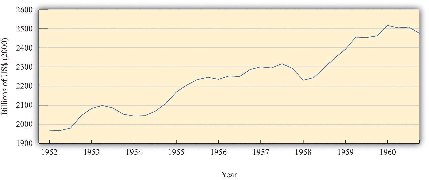
The chart shows real GDP in the United States between 1952 and 1960, measured in billions of year 2000 dollars.
Source: Bureau of Economic Analysis.
This group of economists had, on one hand, a clearly defined goal of stabilizing the macroeconomy and, on the other hand, a set of policy instruments—economic variables such as taxes, government spending, and interest rates—that were under the control of policymakers. They also had a framework of analysis (the aggregate expenditure model) that explained how these instruments could be used to achieve their goals. Finally, they had a president who was willing to listen and take their advice. Never before had economists had such tools and wielded such influence.
The opportunity to test their ideas arose toward the middle of the Kennedy presidency. In the middle of 1962, it was apparent to the Kennedy administration economists that the economy was beginning to sputter. The growth rate of real GDP was 7.1 percent in 1959 but decreased to 2.5 percent and 2.3 percent in 1960 and 1961, respectively.Economic Report of the President (Washington, DC: GPO, 2005):table B-2, GPO Access, accessed September 20, 2011, http://www.gpoaccess.gov/eop/2005/2005_erp.pdf. Their response was to initiate a tax cut.
As is usually the case when a major fiscal policy action is under consideration, there was a lengthy time lag between the initiation of the policy and its implementation. Even though the tax cut was proposed in 1962, President Kennedy never saw it put into effect. He was assassinated in November 1963; the tax cut for individual households and corporations was not enacted until early 1964. For households, tax withholding rates decreased from 18 percent to 14 percent, leading to an estimated tax reduction of about $6.7 billion. Taxes on corporations were also decreased; the reduction in taxes for 1964 was expected to be about $1.7 billion. By 1965, the economists expected that taxes would be lower by $11 billion. In 1965, nominal GDP was about $719 billion, so these changes were about 1.5 percent of nominal GDP.
For many observers of the macroeconomy, this was a watershed event. The Economic Report of the President proclaimed 1965 the “Year of the Tax Cut.” In retrospect, these years were the heyday of Keynesian macroeconomics: for the first time, the government was using tax policy in an attempt to fine-tune the economy.
Figure 27.5 "Tax Policy during the Kennedy Administration" shows what happened to average and marginal tax rates. Marginal tax rates were very high at the time—much greater than in the present day. At high levels of income, more than 90 cents of every additional dollar had to be paid to the government in taxes. Consequently, average tax rates were also high: an individual with taxable income of $100,000 (a very high level of income back then) had to pay about two thirds of that amount to the government. The Kennedy tax cuts reduced these tax rates. Even after the tax cut, the marginal and average tax rates both increased with income. In other words, the tax system still redistributed income across households. But when we compare 1963 and 1964, we see that the marginal tax rate did not increase as rapidly under the new tax policy. Therefore, this channel of redistribution was weaker under the new tax policy.
Figure 27.5 Tax Policy during the Kennedy Administration
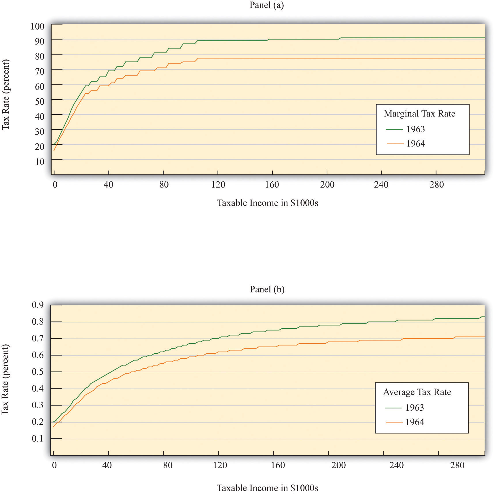
The charts show the impact of the Kennedy tax cut. Part (a) highlights how the marginal tax rates for households changed from 1963 to 1964, and part (b) shows the impact on average tax rates.
Source: Department of the Treasury, IRS 1987, “Tax Rates and Tables for Prior Years” Rev 9-87
For their policy to be successful, Kennedy’s advisors had to ask and then answer a series of questions. How big a tax cut should they recommend? How long should it last? What would be the effect on government revenues? What would be the effect on real GDP and consumption? Economists working in government today confront exactly the same questions when contemplating changes in tax policy. Questions such as these epitomize economics and economists at work.
Looking back at this experiment with almost half a century of hindsight, we can ask additional questions. How well did these policies work in terms of achieving their goal of economic stabilization? What actually happened to consumption and output? Was the tax policy successful?
The Kennedy economists needed a quantitative model of economic behavior: a formalization of the links between their policy tools (tax rates) and the outcomes that they cared about, such as consumption and output. Using the aggregate expenditure model, they wanted to know how big a change in real GDP they could expect from a given change in the tax rate. To use the model to study income taxes, we need to add some theory about how spending responds to changes in taxes. Accordingly, we study the effects of income taxes on household consumption and then discuss how changes in consumption lead to changes in output.
Although we are using a historical episode to help us understand the effect of taxes on the economy, this chapter is not intended as a lesson in economic history. Variations of this same model are still used today to analyze current economic policies. Indeed, in response to the economic crisis of 2008, many countries around the world cut taxes in an attempt to stimulate their economies. By studying the experience of the early 1960s, we gain insight into a critical part of macroeconomics: the linkage between consumption and output.
Having said that, economics has advanced significantly since the 1960s, and the state-of-the-art analysis for that time seems oversimplified today. Modern economists think that the policy advisers in the 1960s neglected some key aspects of the economy. Their insights were not wrong, but they were incomplete. Our understanding of the economy has evolved since Tobin, Solow, and Heller designed the nation’s tax policy.
Household Consumption
We begin by studying the relationship between consumption and income. We first develop some ideas about how households make consumption decisions, and, on the basis of those ideas, we make some predictions about what we expect to happen when there is a cut in taxes. We then examine the evidence from the Kennedy tax cut.
Income, Consumption, and Saving
In microeconomics, we study how a consumer allocates incomes across a wide variety of products. Microeconomists interested in studying, say, the market for ice cream examine how households choose between ice cream and other products that are close substitutes, such as frozen yogurt, and between ice cream and other products that are complements, such as hot fudge sauce. When studying microeconomics, however, we focus on choices for goods made at a particular point in time.
Macroeconomics has a different emphasis. It emphasizes the choice between consumption and saving. Instead of thinking about the consumption of ice cream today versus frozen yogurt today, we study the choice between consumption today and consumption in the future. To highlight this decision, macroeconomists downplay the choices among different goods and services. Of course, in reality, households decide both how much to spend and how much to save, and what products to purchase. But it is convenient to treat these decisions separately.
The same basic ideas of household decision making apply in either case. Households distribute their income across goods to ensure that no redistribution of that spending would make them better off. This is true whether we are talking about ice cream and frozen yogurt, or about consumption and saving. Households allocate their income between consumption and savings in a way that makes them as well off as possible. They do not spend all their income this year because they want to save some for consumption in the future.
Suppose a household in the United States had taxable income of $20,000 in 2010. Some of this income goes to the payment of taxes to federal and state governments. (From our earlier discussion, the average federal tax rate is 13.25 percent.) The rest is either spent on goods and services or saved. The income that is spent on goods and services today is spread over the many products that a household buys. The income that is saved will likewise be used in the future to purchase different goods and services.
Personal Income and Disposable Income
The most basic measure of aggregate economic activity is real GDP, which is the total amount of final goods and services produced in our economy over a period of time, such as a year. The rules of national income accounting mean that real GDP measures three different things at once: the production or output of the economy, the spending in the economy; and the income generated in the economy. We use real GDP as our most general measure of income.
We work in this chapter with two further concepts of income from the national accounts: personal incomeThe income in the economy that flows to households. and disposable incomeIncome after taxes are paid to the government.. Some of the income generated in the economy is retained by firms to finance new investment, so it does not go to households. Personal income refers to that portion of GDP that finds its way directly into the hands of households. (At the level of an individual household, it corresponds closely to adjusted gross income on the tax form.) Disposable income is what remains after we subtract from personal income the taxes paid by households to the government and add to personal income the transfers (such as welfare payments) received by households from the government. For a household, disposable income measures its available resources after taxes have been paid and transfers received.
Consumption Smoothing
Our starting point for understanding consumption choices is the household budget constraint for a typical household. The household receives income from working and other sources and pays taxes to the government. The remainder is the household’s disposable income. The household budget constraint reminds us that, ultimately, you must either spend the income you receive or save it; there are no other choices. That is,
disposable income = consumption + saving.A theory of consumption is a theory of how households decide to divide their income between consumption and saving. Saving is a way to convert current income into future consumption. A theory of consumption is equivalently a theory of saving. A fundamental idea about household behavior is that people do not wish their consumption to vary a lot from month to month or year to year. This principle is so important that economists give it a special name: consumption smoothing. Households use saving and borrowing to smooth out fluctuations in their income and keep their consumption relatively smooth. People will tend to save when their income is high and will dissave when their income is low. (Dissave is the word economists use to mean either running down one’s existing wealth or borrowing against future earnings.)
Toolkit: Section 31.32 "Consumption and Saving"
You can review the consumption-saving decision in the toolkit.
Perfect consumption smoothing means that the household consumes exactly the same amount in each period of time (for example, a month or a year). If a construction worker earns $10,000 per month working from May to October but nothing for the rest of the year, we do not expect that he will spend $10,000 per month in the summer and then starve in the winter. It is much more likely that he will save half of his income in the summer and spend those savings in the winter, so that he spends about $5,000 per month throughout the year.
The logic of consumption smoothing is the same as the argument for why households buy many different goods rather than one single good. Households typically take their income and spend it on a wide variety of products. Furthermore, when income increases, the household will spread this extra income across the spectrum of goods it consumes; not all of it is spent on one good. If you obtain more income, you do not spend all this extra income on ice cream, for example. You buy more of many different goods.
The Consumption Function
One way to represent consumption smoothing is by means of a consumption functionA relationship between current disposable income and current consumption.. This is an equation that relates current consumption to current disposable income. It allows us to go from an abstract idea about consumption behavior—consumption smoothing—to a specific formulation of consumption that we can use in a model of the aggregate economy.
We suppose the consumption function can be represented by the following equation:
consumption = autonomous consumption + marginal propensity to consume × disposable income.-
We make three assumptions:
- Autonomous consumption is positive. Households consume something even if their income is zero. If the household has accumulated a lot of wealth in the past or if the household expects its future income to be larger, autonomous consumption will be larger. It captures both the past and the future.
- We assume that the marginal propensity to consume is positive. The marginal propensity to consume captures the present; it tells us how changes in current income lead to changes in current consumption. Consumption increases as current income increases; the larger the marginal propensity to consume, the more sensitive current spending is to current disposable income. By contrast, the smaller the marginal propensity to consume, the stronger is the consumption-smoothing effect.
- We also assume that the marginal propensity to consume is less than one. This says that not all additional income is consumed. When the household receives more income, it consumes some and saves some. The marginal propensity to save is the amount of additional income that is saved; it equals (1 – marginal propensity to consume).
Table 27.3 "Consumption, Income, and Saving" contains an example of a consumption function where autonomous consumption equals 10,000 and the marginal propensity to consumeThe amount by which consumption increases when disposable income increases by a dollar. equals 0.8. If the household earns no income at all (disposable income = $0), it still spends $10,000 on consumption. In this case, savings equal −$10,000. This means the household is either drawing on existing wealth (accumulated savings from the past) or borrowing against income expected in the future. The marginal propensity to consume tells us how the household divides additional income between consumption and saving. In our example, the household spends 80 percent of any additional income and saves 20 percent.
Table 27.3 Consumption, Income, and Saving
| Disposable Income ($) | Consumption ($) | Saving ($) |
|---|---|---|
| 0 | 10,000 | −10,000 |
| 10,000 | 18,000 | −8,000 |
| 20,000 | 26,000 | −6,000 |
| 30,000 | 34,000 | −4,000 |
| 40,000 | 42,000 | −2,000 |
| 50,000 | 50,000 | 0 |
| 60,000 | 58,000 | 2,000 |
| 70,000 | 66,000 | 4,000 |
| 80,000 | 74,000 | 6,000 |
| 90,000 | 82,000 | 8,000 |
| 100,000 | 90,000 | 10,000 |
For example, when income is equal to $20,000, consumption can be calculated as follows:
consumption = $10,000 + 0.8 × $20,000 = $10,000 + 0.8 × $20,000 = $26,000.The household is still dissaving but now only by $6,000. Table 27.3 "Consumption, Income, and Saving" also shows that when income equals $50,000, consumption and income are equal, so savings are exactly zero. At income levels above $50,000, the household has positive savings.
Figure 27.6 "Consumption, Saving, and Income" shows the relationship between consumption and income graphically. We also graph the savings function in Figure 27.6 "Consumption, Saving, and Income". The savings function has a negative intercept because when income is zero, the household will dissave. The savings function has a positive slope because the marginal propensity to saveThe amount by which saving increases when disposable income increases by a dollar. is positive.
Figure 27.6 Consumption, Saving, and Income
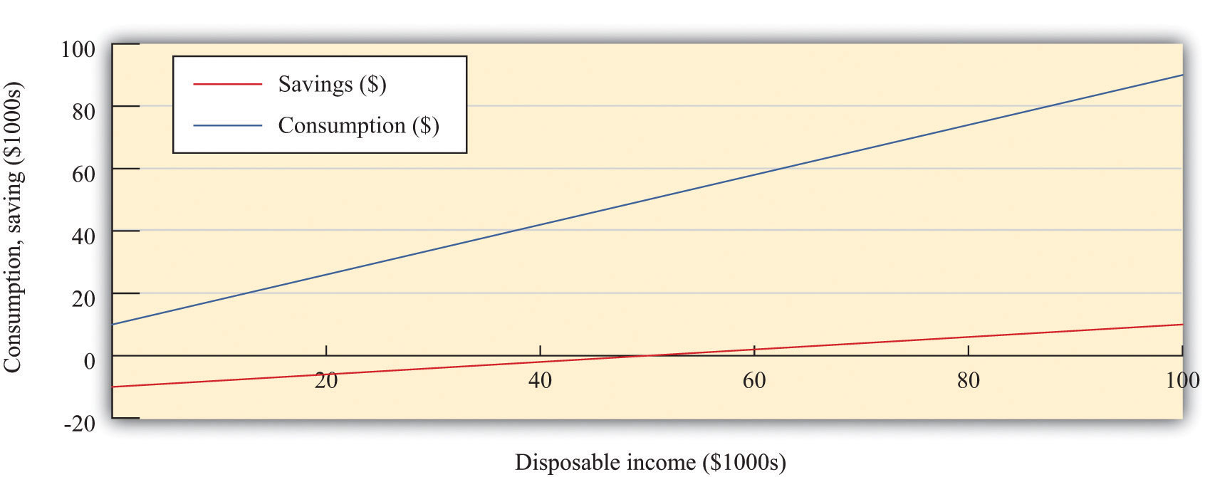
The graph shows the relationship between consumption and disposable income, where autonomous consumption is $10,000 and the marginal propensity to consume is 0.8. When disposable income is below $50,000, savings are negative, whereas at income levels above $50,000, savings are positive.
As well as the marginal propensity to consume and the marginal propensity to save, we can examine the average propensity to consumeThe ratio of consumption to disposable income., which measures how much income goes to consumption on average. It is calculated as follows:
When disposable income increases, consumption increases but by a smaller amount. This means that when disposable income increases, people consume a smaller fraction of their income: the average propensity to consume decreases.In terms of mathematics, we are saying that, if we divide through the consumption function by disposable income, we getAn increase in disposable income reduces the first term and the average propensity to consume. Meanwhile, the ratio of saving to disposable income is called the savings rateThe ratio of household savings to disposable income.. For example,
The savings rate and the average propensity to consume together sum to 1. In other words, a decline in the average propensity to consume equivalently means that households are saving a larger fraction of their income.
Because the consumption and savings relationships are two sides of the same coin, economists wishing to find the actual values of autonomous consumption and the marginal propensity to consume can examine data on consumption, savings, or both. If the data were perfect, we would get the same answer either way. For the United States, both consumption and savings data are readily available, but in some countries the data on savings may be of higher quality than the consumption data, in which case economists use savings data to understand consumption behavior.
Some Warnings about the Consumption Function
The consumption function is useful because it captures two fundamental insights: households seek to smooth their consumption, but consumption nonetheless responds to current income. But the consumption function is really too simple.Refining our theory of consumption is a subject for Chapter 28 "Social Security".
First, it ignores the role of accumulated wealth. If you consider two households with the same level of current income but different amounts of accumulated wealth, the one with higher wealth will probably consume more. Second, the consumption function does not explicitly include the role of expectations. A household’s consumption reflects not only income today and the accumulation of income in the form of wealth but also anticipated income. So, for example, if a government announces that it will increase income tax rates in two years, we expect that households will respond immediately to smooth out the effects of these future taxes. The only way the consumption function allows us to capture wealth or expectations of future income is through autonomous consumption. This is fine as far as it goes, but it means that we are taking too many aspects of consumption as given, rather than explaining them with our theory.
Another complication is that changes in income today are often correlated with changes in income in the future. If your income increases today, is this an indication that your income will also be higher in the future? To see why this matters, consider two extreme examples. First, suppose that you receive a one-time inheritance of $10 million. What will you do with this income? According to the consumption smoothing argument, you will save some of this income to increase your consumption in the future. Roughly speaking, if you thought you had 10 years left to live, you might increase your consumption by about $1 million per year. In this case your marginal propensity to consume would be only 0.1.
Now suppose that instead of a $10 million windfall, you learn you will receive $1 million each year for the next 10 years. In this case, your income is already spread out over your lifetime. So, in this second case, you will again want to smooth your consumption. But since the increase in income will be maintained for your lifetime, you can increase your consumption by an amount equal to the increase in your income. Your marginal propensity to consume will be 1.0.
The difference between these two situations is that in the first case the income increase is temporary, and in the second it is permanent. The logic of consumption smoothing implies that the marginal propensity to consume is near 1 for permanent changes in income but much smaller for temporary changes in income.
The Effects of a Change in Income Taxes
We can now figure out the effects of a cut in taxes on consumption and saving. A reduction in taxes will increase disposable income. From the consumption function, this results in an increase in consumption equal to the marginal propensity to consume times the increase in disposable income. The average propensity to consume decreases. To summarize, if taxes are cut in the economy, we expect to see the following:
- An increase in disposable income
- An increase in consumption that is smaller than the increase in disposable income (that is, a marginal propensity to consume less than 1)
- A decline in the average propensity to consume
When natural scientists such as molecular biologists or particle physicists want to see how good their theories are, they conduct experiments. Economists and other social scientists have much less ability to carry out experiments—certainly at the level of the macroeconomy. The Kennedy tax cut, however, is like a “natural” experiment in that there was a major policy change that we can think of as a change in an exogenous variableA variable determined outside the model that is not explained in the analysis.. It is not, in truth, completely exogenous. We already explained that the tax cut was enacted in response to the poor performance of the economy. We are not badly misled by thinking of it as an exogenous event, however. We can therefore use it to see how well our theory performs. Specifically, we can look to see whether disposable income and consumption do behave as we have predicted.
Empirical Evidence on Consumption
Before we turn to those specific questions, let us examine some data on consumption. Figure 27.7 "Consumption and Income" shows the behavior of consumption and disposable income from 1962 to 2010. The measures of both income and consumption are in year 2005 dollars. This means that the nominal (money) levels of income and consumption for each of the years have been corrected for inflation, so that we can see how the real level of consumption relates to the real level of income.
Figure 27.7 Consumption and Income
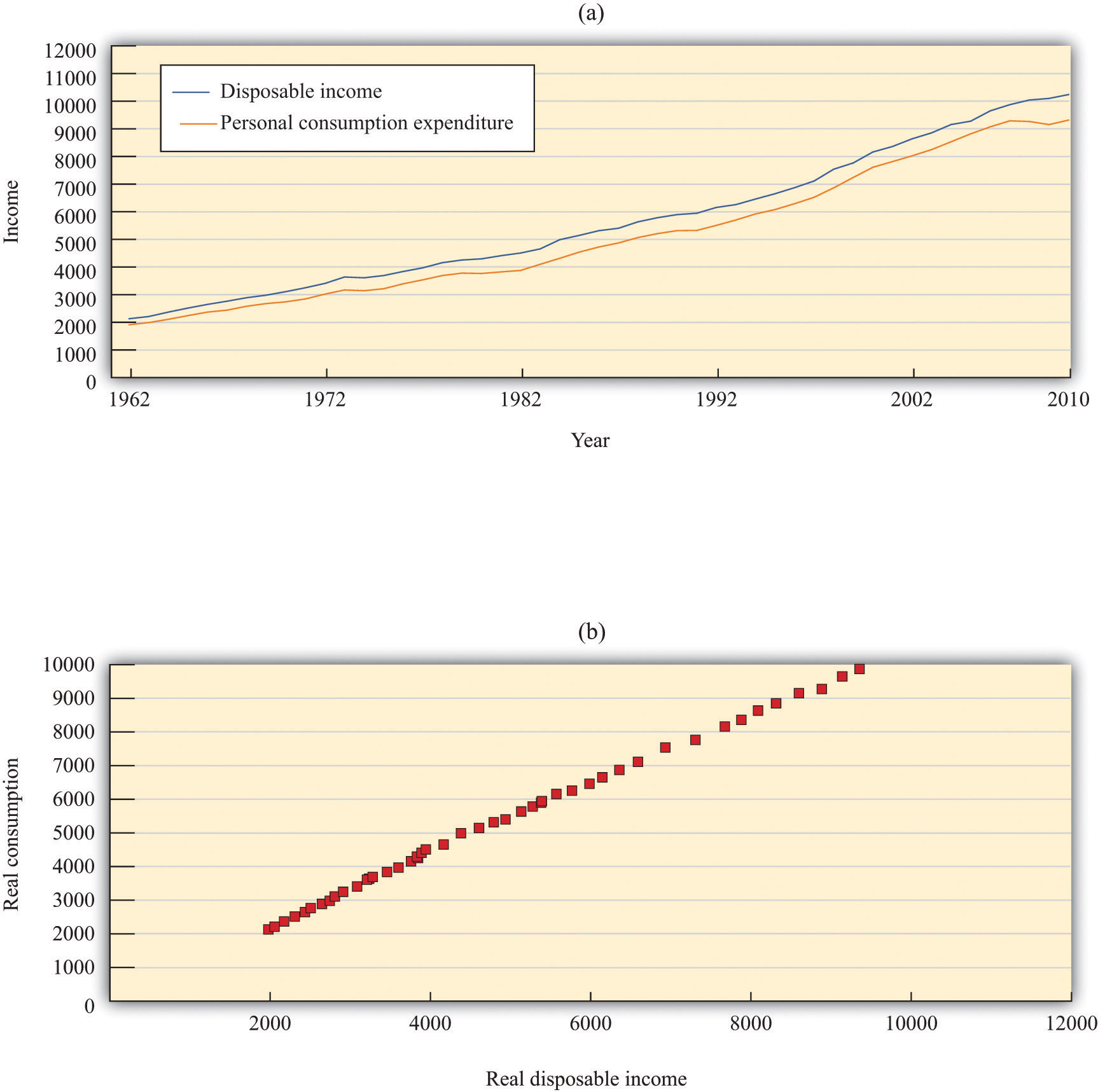
The charts show consumption and personal disposable income (in billions of year 2005 dollars) from 1962 to 2010. Consumption and disposable income grew substantially over this time (a) and there is a close relationship between consumption and income (b).
Source: Economic Report of the President (Washington, DC: GPO, 2011), table B-31, accessed September 20, 2011, http://www.gpoaccess.gov/eop/tables11.html.
Toolkit: Section 31.8 "Correcting for Inflation"
You can review how to correct for inflation in the toolkit.
The first thing we see in Figure 27.7 "Consumption and Income" is that both consumption and disposable income grew substantially over the 1962–2010 period. This should come as no surprise. We know that the US economy grew over this period, so we would expect that disposable income and consumption would also grow. Figure 27.7 "Consumption and Income" reveals that, as a consequence, there is a close relationship between consumption and income, and consumption expenditures are, on average, about 91 percent of disposable income. Although Figure 27.7 "Consumption and Income" looks something like a consumption function, we should not take this relationship as strong evidence for our theory because it is primarily caused by the fact that both variables grew over time.
Consumption Response to the Kennedy Tax Cut
Now we return to the Kennedy tax cut. How well does our model perform in predicting the effects of the tax changes on consumption? Superficially, this seems like an easy question. We can examine the changes in consumption and income that arose after the tax changes and see whether these changes are consistent with the model.
There is a critical difference between our theory and reality, however. When we discussed the effects of a tax cut using our theory, we implicitly held everything else constant. We presumed that there was a change in taxes and no change in any other variable. For example, we assumed that government spending, investment spending, and net exports all did not change. In fact, other economic variables were changing at the same time that the new tax policy went into effect; these changes could also have affected consumption and disposable income. Looking at particular tax experiments is a messy business.
Taxes were cut in February 1964, and (real) disposable income increased by $430 billion, a much larger increase than in previous time periods. Consumption expenditures increased considerably during this period. Table 27.4 "Consumption and Income in the 1960s (Seasonally Adjusted, Annual Rates)" summarizes the behavior of GDP, disposable income, consumption, and the average propensity to consume over the 1960–68 period. Remember that these are real variables, measured in year 2000 dollars. The average propensity to consume is calculated as consumption divided by disposable income, and the marginal propensity to consume is calculated as the change in consumption divided by the change in disposable income.
Table 27.4 Consumption and Income in the 1960s (Seasonally Adjusted, Annual Rates)
| Year | Real GDP ($) | Disposable Income ($) | Consumption ($) | APC | MPC |
|---|---|---|---|---|---|
| 1960 | 2,501.8 | 1,759.7 | 1,597.4 | 0.91 | — |
| 1961 | 2,560.0 | 1,819.2 | 1,630.3 | 0.90 | 0.55 |
| 1962 | 2,715.2 | 1,908.2 | 1,711.1 | 0.90 | 0.91 |
| 1963 | 2,834.0 | 1,979.1 | 1,781.6 | 0.90 | 0.99 |
| 1964 | 2,998.6 | 2,122.8 | 1,888.4 | 0.89 | 0.74 |
| 1965 | 3,191.1 | 2,253.3 | 2,007.7 | 0.89 | 0.97 |
| 1966 | 3,399.1 | 2,371.9 | 2,121.8 | 0.89 | 0.96 |
| 1967 | 3,484.6 | 2,475.9 | 2,185.0 | 0.88 | 0.61 |
| 1968 | 3,652.7 | 2,588.0 | 2,310.5 | 0.89 | 1.11 |
| APC, average propensity to consume; MPC, marginal propensity to consume. | |||||
Source: Economic Report of the President (Washington, DC: GPO 2004), accessed September 20, 2011, http://www.gpoaccess.gov/eop.
Disposable income increased as did consumption, in accordance with the predictions of our theory. As the theory predicts, the average propensity to consume decreased for most of this period. Likewise, in line with the theory, the marginal propensity to consume was less than 1 (in all years except 1968). Thus the evidence from this period is broadly consistent with the predictions that we made on the basis of our model.
Aggregate Income, Aggregate Consumption, and Aggregate Saving
The 1964 tax cut was not designed to influence consumption in isolation but rather to have an impact on the overall economy via its effect on consumption. So far, we have argued that a change in taxes leads to a change in disposable income and hence a change in consumption. Now we complete the story, noting that a change in consumption will itself affect the level of real GDP and hence have further effects on the level of disposable income.
In the case of the Kennedy tax cut of 1964, the economists advising the administration at that time had a fairly specific idea of how changes in consumption would affect the overall economy. They argued that the $10 billion tax cut would lead to an increase in GDP of about $20 billion each year. How did they create this estimate? To answer this question, we need to embed our theory of consumption in the aggregate expenditure model.
We motivated our consumption function by thinking about the behavior of an individual household. We now presume that our household is in some sense average, or representative of the entire economy, so the consumption relationship holds at an economy-wide level. Different households might actually have different consumption functions, but when we add them together, we still expect to find an aggregate relationship similar to the one we have described.
The economists of the time used a framework that was closely based on the aggregate expenditure model. When prices are sticky, the level of GDP is determined in that model by the condition that planned spending and actual spending are equal. The model tells us that the level of real GDP depends on the level of autonomous spending and the multiplier,
real GDP = multiplier × autonomous spending,where the multiplier is calculated as Given the level of autonomous spending in the economy and given a value for the marginal propensity to spend, we can calculate the equilibrium level of real GDP.
The marginal propensity to spend is not the same thing as the marginal propensity to consume, although they are connected. The marginal propensity to spend tells us how much total spending changes when GDP changes. Total spending includes not only consumption but also investment, government purchases, and net exports, so if any of these are responsive to changes in GDP, then the marginal propensity to spend is affected. Likewise, autonomous spending is not the same as autonomous consumption. Autonomous spending is the sum of autonomous consumption, autonomous investment, autonomous government purchases, and autonomous net exports. Finally, the marginal propensity to consume measures how consumption responds to changes in disposable income, not GDP.
Toolkit: Section 31.30 "The Aggregate Expenditure Model"
You can review the aggregate expenditure model and the multiplier in the toolkit.
In our analysis here, we continue to focus on consumption and suppose that the other components of spending—government spending, investment, and net exports—are exogenous. That is, these variables are all unaffected by changes in income and so are all included in autonomous spending. In addition, we presume that the amount that the government spends is not affected by the amount that it receives in tax revenue.
To find out the effects on the economy of a change in income taxes, we take the equation for real GDP and write it in terms of changes:
change in real GDP = multiplier × change in autonomous spending.This equation tells us we need two pieces of information to work out the effect of a tax change:
- The marginal propensity to spend because this allows us to calculate the multiplier
- The effect of a tax change on autonomous spending
Let us think about the marginal propensity to spend first. We want to know the answer to the following question: if GDP changes by some amount (say, $100), what will happen to spending? There are three pieces to the answer.
- A change in GDP leads to a change in personal income. Remember from the circular flow of income that GDP measures production, income, and expenditure in the economy. Firms receive income when they sell their products. Most of that income finds its way into the hands of households in the form of wage and salary payments or dividend payments. Firms hold onto some of the income that they generate, however, to replace worn-out capital goods and finance new investments. In the early 1960s, personal income was about 78 percent of GDP. So if GDP increased by $100, we would expect personal income to increase by about $78.
- A change in personal income leads in turn to a change in disposable income. As we explained at length, personal income is taxed, so disposable income is less than personal income. Since we are considering the effects of a change in taxes, we need an estimate of the marginal tax rate facing consumers. We know from Figure 27.3 that this varied across individuals, but researchers have estimated that, for the economy as a whole, the marginal tax rate in 1964 was about 22 percent.Robert J. Barro and Chaipat Sasakahu provide estimates of the “average marginal tax rate.” Barro and Sasakahu, “Measuring the Average Marginal Tax Rate from the Individual Income Tax” (NBER Working Paper No. 1060 [Reprint No. r0487], June 1984), http://www.nber.org/papers/w1060. To put it another way, households would keep about 78 percent (= 100 percent – 22 percent) of their personal income. So if personal income increased by $78, disposable income would increase by about $61 (= 0.78 × $78). (It is a meaningless coincidence that these two numbers are both 78 percent.)
- Finally, a change in disposable income leads to a change in consumption. According to the 1964 Economic Report of the President, the CEA thought that the marginal propensity to consume was about 0.93. So if disposable income increased by $61, we would expect consumption to increase by about $57 (= 0.93 × $61).
Putting these three together, therefore, we see that an increase in GDP of $100 causes consumption to increase by $57. The marginal propensity to spend in this economy was equal to about 57 percent. It follows that the CEA thought that the multiplier was equal to about 2.3 because
Now let us think about the change in autonomous spending. We have said that taxes were cut by about $10 billion. We expect that most of this tax cut ended up in the hands of consumers. Based on the marginal propensity to consume of 0.93, we would therefore expect there to be an increase of about $9.3 billion in autonomous consumption,
change in autonomous spending = $9.3 billion.Putting these two results together, we find that our prediction for the change in GDP as a result of the tax cut is
change in real GDP = multiplier × change in autonomous spending = 2.3 × $9.3 billion = $21.4 billion.Our answer is not exactly equal to the $20 billion predicted by the CEA, but it is very close. As you might expect, the CEA was working with a more complicated model than the one we have explained here, and, as a result, they came up with a slightly smaller number for the multiplier.
A Word of Warning
All our analysis so far has ignored the fact that, through the price adjustment equation, increased real GDP causes the price level to rise. This increase in prices serves to choke off some of the effects of the increase in spending. In effect, we have ignored the supply side of the economy. It is not that the Kennedy-Johnson administration economists were naïve about the supply side, but they thought the demand side movements were much more relevant for short-run policymaking purposes. More recent economic experience has convinced economists that we ignore the supply side of the economy at our peril. Modern macroeconomists would be careful to augment this story with a discussion of price adjustment.
Toolkit: Section 31.31 "Price Adjustment"
You can review price adjustment in the toolkit.
Key Takeaways
- Beginning in the early 1960s, growth of real GDP began to slow. This provided the basis for the tax cut of 1964.
- The CEA economists used the aggregate expenditure model as the basis for their analysis of the effects of the tax cut.
- In response to the tax cut, consumption and real GDP both increased. This fits with the prediction of the aggregate expenditure model.
Checking Your Understanding
- Is the marginal propensity to consume independent of whether an income increase is viewed as temporary or permanent?
- If autonomous consumption is positive, is the level of savings at zero disposable income positive or negative?