Appendix: Forecasting

This is “Appendix: Forecasting”, section 4.6 from the book Enterprise and Individual Risk Management (v. 1.0). For details on it (including licensing), click here.

For more information on the source of this book, or why it is available for free, please see the project's home page. You can browse or download additional books there. To download a .zip file containing this book to use offline, simply click here.

Has this book helped you? Consider passing it on:

Help Creative Commons

Creative Commons supports free culture from music to education. Their licenses helped make this book available to you.

Help a Public School

DonorsChoose.org helps people like you help teachers fund their classroom projects, from art supplies to books to calculators.

4.6 Appendix: Forecasting

Forecasting of Frequency and Severity

When insurers or risk managers use frequency and severity to project the future, they use trending techniques that apply to the loss distributions known to them.Forecasting is part of the Associate Risk Manager designation under the Risk Assessment course using the book: Baranoff Etti, Scott Harrington, and Greg Niehaus, Risk Assessment (Malvern, PA: American Institute for Chartered Property Casualty Underwriters/Insurance Institute of America, 2005). Regressions are the most commonly used tools to predict future losses and claims based on the past. In this textbook, we introduce linear regression using the data featured in Chapter 2 "Risk Measurement and Metrics". The scientific notations for the regressions are discussed later in this appendix.

Table 4.5 Linear Regression Trend of Claims and Losses of A

Year	Actual Fire Claims	Linear Trend For Claims	Actual Fire Losses	Linear Trend For Losses
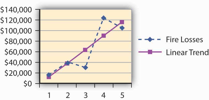
1	11	8.80	$16,500	$10,900.00
2	9	9.50	$40,000	$36,900.00
3	7	10.20	$30,000	$62,900.00
4	10	10.90	$123,000	$88,900.00
5	14	11.60	$105,000	$114,900.00

Figure 4.5 Linear Regression Trend of Claims of A

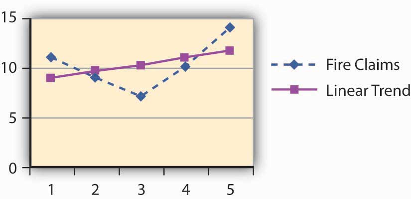
Figure 4.6 Linear Regression Trend of Losses of A

Using Linear Regression

Linear regression attempts to explain the relationship among observed values by applying a straight line fit to the data. The linear regression model postulates that

Y = b + m X + e

,where the “residual” e is a random variable with mean of zero. The coefficients a and b are determined by the condition that the sum of the square residuals is as small as possible. For our purposes, we do not discuss the error term. We use the frequency and severity data of A for 5 years. Here, we provide the scientific notation that is behind Figure 4.5 "Linear Regression Trend of Claims of A" and Figure 4.6 "Linear Regression Trend of Losses of A".

In order to determine the intercept of the line on the y-axis and the slope, we use m (slope) and b (y-intercept) in the equation.

Given a set of data with n data points, the slope (m) and the y-intercept (b) are determined using:

m = \frac{n Σ (x y) - Σ x Σ y}{n Σ (x^{2}) - {(Σ x)}^{2}}

b = \frac{Σ y - m Σ x}{n}

Figure 4.7 Showing the Slope and Intercept

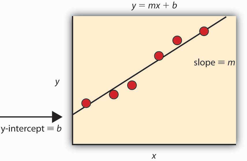
The graph is provided by Chris D. Odom, with permission.

Most commonly, practitioners use various software applications to obtain the trends. The student is invited to experiment with Microsoft Excel spreadsheets. Table 4.6 "Method of Calculating the Trend Line for the Claims" provides the formulas and calculations for the intercept and slope of the claims to construct the trend line.

Table 4.6 Method of Calculating the Trend Line for the Claims

	(1)	(2)	(3) = (1) × (2)	(4) = (1)2
	Year	Claims
	X	Y	XY	X2
	1	11	11.00	1
	2	9	18.00	4
	3	7	21.00	9
	4	10	40.00	16
	n=5	14	70.00	25
Total	15	51	160	55
M = Slope = 0.7	= $m = \frac{n Σ (x y) - Σ x Σ y}{n Σ (x^{2}) - {(Σ x)}^{2}}$			$= \frac{(5 \times 160) - (15 \times 51)}{(5 \times 55) - (15 \times 15)}$
b = Intercept = 8.1	$b = \frac{Σ y - m Σ x}{n}$			$= \frac{51 - (0.7 \times 15)}{5}$

Future Forecasts using the Slopes and Intercepts for A:

Future claims = Intercept + Slope × (X)
In year 6, the forecast of the number of claims is projected to be: {8.1 + (0.7 × 6)} = 12.3 claims

Future losses = Intercept + Slope × (X)
In year 6, the forecast of the losses in dollars is projected to be: {−15, 100 + (26,000 × 6)} = $140,900 in losses

The in-depth statistical explanation of the linear regression model is beyond the scope of this course. Interested students are invited to explore statistical models in elementary statistics textbooks. This first exposure to the world of forecasting, however, is critical to a student seeking further study in the fields of insurance and risk management.