This is “Chapter Assignments and Tests”, section 3.4 from the book Using Microsoft Excel (v. 1.1). For details on it (including licensing), click here.
For more information on the source of this book, or why it is available for free, please see the project's home page. You can browse or download additional books there. To download a .zip file containing this book to use offline, simply click here.


3.4 Chapter Assignments and Tests
To assess your understanding of the material covered in the chapter, please complete the following assignments.
Careers in Practice (Skills Review)
Retail Inventory Analyst (Comprehensive Review Part A)
Starter File: Chapter 3 CiP Exercise 1
Difficulty: Level 1 Easy
The challenge of pursuing any position in a retail career is analyzing large volumes of data to measure the financial performance of the business. Large retail corporations may service thousands of customers in hundreds of stores every day. This creates an enormous amount of sales data that is typically stored in large database systems. A retail analyst is typically asked to make sense of all this data and develop reports for other managers in the company. In fact, a retail analyst is often asked to prepare sales reports for the most senior executives in a retail corporation. The skills covered in this chapter are extremely valuable in helping a retail analyst summarize large volumes of data that allow other managers to understand the financial performance of the company and make critical decisions every day. In this exercise, you will create a sales report similar to one that is commonly used in a retail career. This part of the exercise utilizes the IF function to analyze the sales and inventory data by store. The information created from this analysis can be shared with a manager in the shipping department. Begin this exercise by opening the file named Chapter 3 CiP Exercise 1.
- Click cell D3 on the Sales by Store worksheet. Set the Freeze Panes command by clicking the View tab of the Ribbon and then clicking the Freeze Panes button. Select the Freeze Panes option from the drop-down list. This will keep the column headings and store numbers in view as you scroll through the worksheet.
-
Click cell L3 on the Sales by Store worksheet. Enter an IF function by typing an equal sign (=) followed by the function name IF and an open parenthesis ((). Define the arguments of the function as follows:
- Logical_test: The logical test will assess if the value in cell J3 is greater than 5%. Click cell J3 and then type >5%. Complete the argument by typing a comma.
- Value_if_true: If the logical test is true, the function should show the word Growth. Type the word “Growth” with the quotation marks as shown. Complete the argument by typing a comma.
- Value_if_false: If the logical test is false, the function should leave the cell blank. To do this, type two quotation marks (“”). Complete the function by typing a closing parenthesis and press the ENTER key on your keyboard.
-
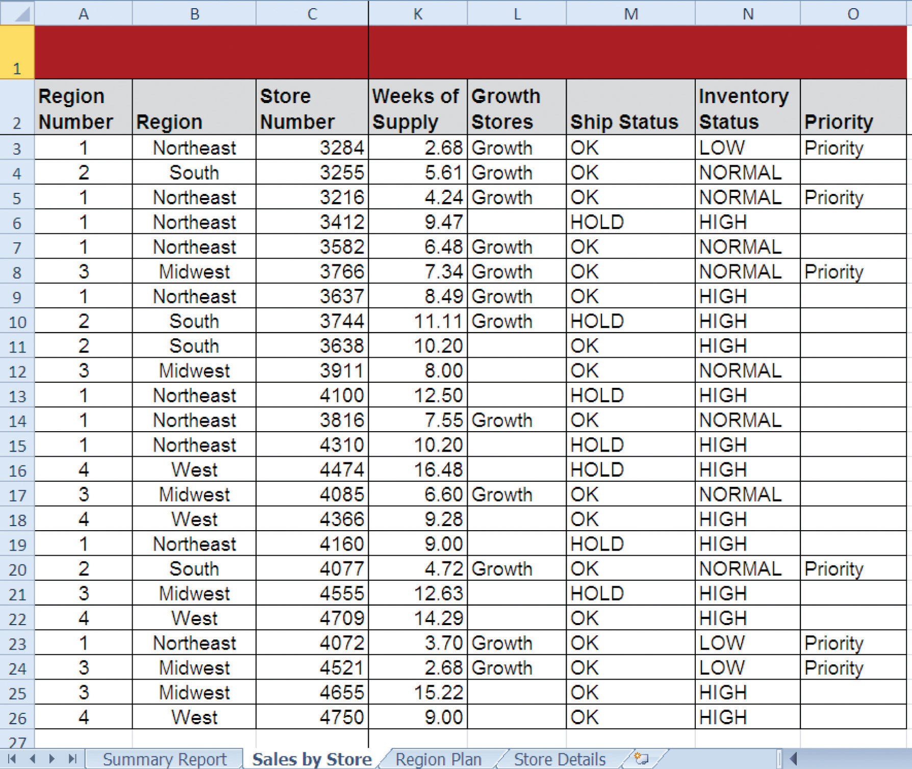
Copy and paste the IF function in cell L3 into the range L4:L26 by double clicking the Auto Fill Handle (see Figure 3.54). You will see the word Growth only for stores where sales are growing at a rate greater than 5% compared to last year. The other cell locations in this column will remain blank if the growth rate is at or less than 5%.
Figure 3.54
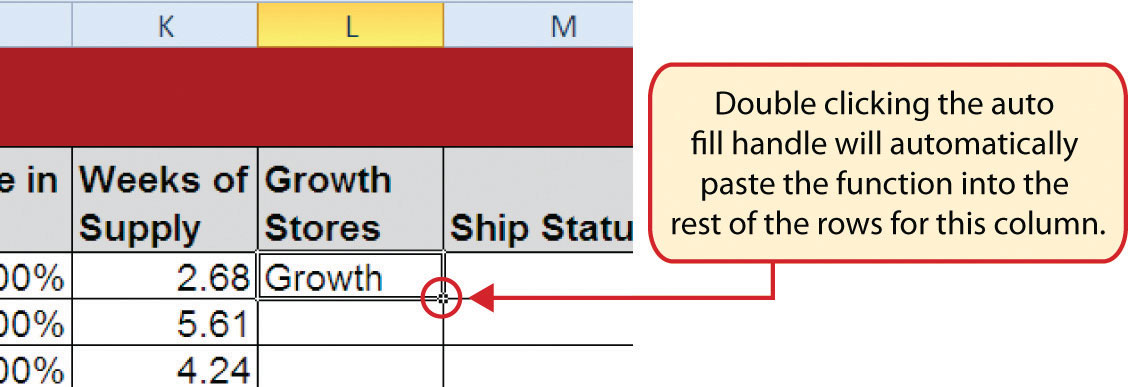
Double click the Auto Fill Handle to copy and paste formulas and functions.
-
Click cell M3 on the Sales by Store worksheet. This column will use the AND function within the IF function to identify small stores that cannot receive any shipments until more inventory is sold. Begin the function by typing an equal sign (=) followed by the function name IF and an open parenthesis ((). Define the arguments of the function as follows:
- Logical_test: The logical test will assess if the store size in cell F3 is equal to 10000 and if the weeks of supply in cell K3 is greater than 8. This will require the use of the AND function. Type the function name AND followed by an open parenthesis. Define the first argument by clicking cell F3 and then typing the following: =10000. Type a comma and define the second argument by clicking cell K3 and then typing the following: >8. Type a closing parenthesis followed by a comma (),).
- Value_if_true: If the logical test is true, the function should show the word HOLD. Type “HOLD” with the quotation marks as shown. Complete the argument by typing a comma.
- Value_if_false: If the logical test is false, the function should show the word OK. Type “OK” with the quotation marks as shown. Complete the function by typing a closing parenthesis and press the ENTER key on your keyboard.
- Copy and paste the IF function in cell M3 into the range M4:M26 by double clicking the Auto Fill Handle. The function now shows for any store that is 10,000 square feet if shipments should be held.
-
Click cell N3 on the Sales by Store worksheet. This column will show for all stores if the inventory is too high, low, or normal. This will require a nested IF function. Begin the function by typing an equal sign (=) followed by the function name IF and an open parenthesis ((). Define the arguments of the function as follows:
- Logical_test: The first logical test will assess if the weeks of supply in cell K3 is less than 4. Click cell K3 and then type <4. Complete the argument by typing a comma.
- Value_if_true: If the logical test is true, the function should show the word LOW. Type “LOW” with the quotation marks as shown. Complete the argument by typing a comma.
- Value_if_false: This argument will be used to begin a second IF function. Type the function name IF and an open parenthesis ((). Define the arguments of this second IF function as follows:
- Logical_test: This second logical test will assess if the weeks of supply in cell K3 is greater than 8. Click cell K3 and then type >8. Complete the argument by typing a comma.
- Value_if_true: If the logical test is true, the function should show the word HIGH. Type “HIGH” with the quotation marks as shown. Complete the argument by typing a comma.
- Value_if_false: IF the second logical test is false, the function should show the word NORMAL. Type “NORMAL” with the quotation marks as shown. Complete the function by typing two closing parentheses ())).Press the ENTER key.
- Copy and paste the IF function in cell N3 into the range N4:N26 by double clicking the Auto Fill Handle. The function now highlights for each store if the inventory is low, high, or normal.
-
Click cell O3 on the Sales by Store worksheet. This column will use the OR function within the IF function to identify stores that should be prioritized for merchandise shipments. Begin the function by typing an equal sign (=) followed by the function name IF and an open parenthesis ((). Define the arguments of the function as follows:
- Logical_test: The logical test will assess if the change in sales in cell J3 is greater than 8% or if the weeks of supply in cell K3 is less than 5. This will require the use of the OR function. Type the function name OR followed by an open parenthesis ((). Define the first argument by clicking cell J3 and then typing the following: >8%. Type a comma and define the second argument by clicking cell K3 and then typing the following: <5. Type a closing parenthesis followed by a comma (),).
- Value_if_true: If the logical test is true, the function should show the word Priority. Type “Priority” with the quotation marks as shown. Complete the argument by typing a comma.
- Value_if_false: If the logical test is false, the function should leave the cell blank. To do this, type two quotation marks (“”). Complete the function by typing a closing parenthesis and press the ENTER key on your keyboard.
- Copy and paste the IF function in cell O3 into the range O4:O26 by double clicking the Auto Fill Handle. The function now shows the word Priority for any store that is experiencing high sales growth or low inventory. This information can also be used by a shipping manager to prioritize the flow of deliveries to the stores.
- Save the workbook by adding your name in front of the current workbook name (i.e., “your name Chapter 3 CiP Exercise 1”).
- Close the workbook and Excel.
Figure 3.55 Completed CiP Exercise 1 Sales by Store Worksheet (Columns L–O)
Careers in Practice (Skills Review)
Retail Sales Analyst (Comprehensive Review Part B)
Starter File: Chapter 3 CiP Exercise 1 (Continued from Comprehensive Review Part A)
Difficulty: Level 2 Moderate
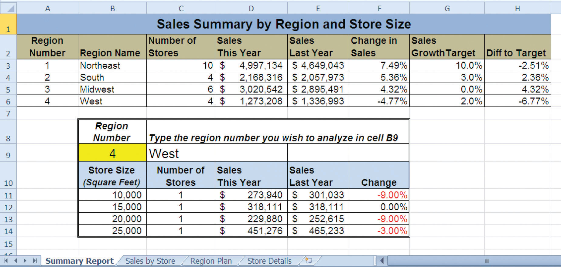
This exercise continues the career theme for a retail analyst. In this exercise, you will summarize the detailed sales data using the statistical IF functions. The report will summarize the store level detail by region, which could be used by senior executives of the company. Begin this exercise by opening the file named Chapter 3 CiP Exercise 1 or continue with this file if you completed the comprehensive review part A.
-
Click cell C3 on the Summary Report worksheet. This column will be used to count the stores for each region of the company. Begin the function by clicking the Formulas tab on the Ribbon. Click the More Functions button, click the Statistical option, and then click the COUNTIF function from the list. Define the arguments in the Function Arguments dialog box as follows:
- Range: Click the Collapse Dialog button next to the Range argument, click the Sales by Store worksheet tab, and highlight the range A3:A26. Press the ENTER key on your keyboard. Click in the input box for the Range argument and place an absolute reference on the range. Press the TAB key on your keyboard to advance to the next argument.
- Criteria: Type cell A3. Complete the function by clicking the OK button at the bottom of the Function Arguments dialog box.
- Copy and paste the COUNTIF function in cell C3 by double clicking the Auto Fill Handle. The function will show the number of stores for each region.
-
Click cell D3 on the Summary Report worksheet. This column will be used to sum the current sales by region. Begin the function by clicking the Formulas tab on the Ribbon. Click the Math & Trig button and select the SUMIF function from the list. Define the arguments in the Function Arguments dialog box as follows:
- Range: Click the Collapse Dialog button next to the Range argument, click the Sales by Store worksheet tab, and highlight the range A3:A26. Press the ENTER key on your keyboard. Click in the input box for the Range argument and place an absolute reference on the range. Press the TAB key on your keyboard to advance to the next argument.
- Criteria: Type cell A3. Press the TAB key on your keyboard to advance to the next argument.
- Sum_range: Click the Collapse Dialog button next to the Sum_range argument, click the Sales by Store worksheet tab, and highlight the range I3:I26. Press the ENTER key on your keyboard. Click in the input box for the Sum_range argument and place an absolute reference on the range. Complete the function by clicking the OK button at the bottom of the Function Arguments dialog box.
- Copy and paste the SUMIF function in cell D3 by double clicking the Auto Fill Handle. The function will show the total sales this year for each region.
- Click cell E3 on the Summary Report worksheet. This column will be used to sum the sales last year by region. Enter a SUMIF function and define the arguments exactly as stated in step 3. However, define the Sum_range argument with the range H3:H26 on the Sales by Store worksheet. Remember to put an absolute reference on this range before completing the function.
- Copy and paste the SUMIF function in cell E3 by double clicking the Auto Fill Handle. The function will show the total sales last year for each region.
- Enter a formula in cell F3 on the Summary Report worksheet to calculate the percent change in sales for each region. Your formula should first subtract the Sales Last Year in cell E3 from the Sales This Year in cell D3. Then divide this result by the Sales Last Year in cell E3.
- Copy and paste the formula in cell F3 by double clicking the Auto Fill Handle.
-
Click cell C11 on the Summary Report worksheet. This column will be used to count the number of stores by size for the region number typed into cell B9. Begin the function by clicking the Formulas tab on the Ribbon. Click the More Functions button, click the Statistical option, and select the COUNTIFS function from the list. Define the arguments in the Function Arguments dialog box as follows:
- Criteria_range1: Click the Collapse Dialog button next to the Criteria_range1 argument, click the Sales by Store worksheet tab, and highlight the range A3:A26. Press the ENTER key on your keyboard. Click in the input box for the Criteria_range1 argument and place an absolute reference on the range. Press the TAB key on your keyboard to advance to the next argument.
- Criteria1: Type cell B9. Place an absolute reference on this cell location. Press the TAB key on your keyboard to advance to the next argument.
- Criteria_range2: Click the Collapse Dialog button next to the Criteria_range2 argument, click the Sales by Store worksheet tab, and highlight the range F3:F26. Press the ENTER key on your keyboard. Click in the input box for the Criteria_range2 argument and place an absolute reference on the range. Press the TAB key on your keyboard to advance to the next argument.
- Criteria2: Type cell B11. Complete the function by clicking the OK button at the bottom of the Function Arguments dialog box.
- Copy the COUNTIFS function in cell C11 and paste it into the range C12:C14 using the Paste Formulas command.
-
Click cell D11 on the Summary Report worksheet. This column will be used to sum the current sales by store size for the region number typed into cell B9. Begin the function by clicking the Formulas tab on the Ribbon. Click the Math & Trig button, and select the SUMIFS function from the list. Define the arguments in the Function Arguments dialog box as follows:
- Sum_range: Click the Collapse Dialog button next to the Sum_range argument, click the Sales by Store worksheet tab, and highlight the range I3:I26. Press the ENTER key on your keyboard. Click in the input box for the Sum_range argument and place an absolute reference on the range. Press the TAB key on your keyboard to advance to the next argument.
- Criteria_range1: Click the Collapse Dialog button next to the Criteria_range1 argument, click the Sales by Store worksheet tab, and highlight the range A3:A26. Press the ENTER key on your keyboard. Click in the input box for the Criteria_range1 argument and place an absolute reference on the range. Press the TAB key on your keyboard to advance to the next argument.
- Criteria1: Type cell B9. Place an absolute reference on this cell location. Press the TAB key on your keyboard to advance to the next argument.
- Criteria_range2: Click the Collapse Dialog button next to the Criteria_range2 argument, click the Sales by Store worksheet tab, and highlight the range F3:F26. Press the ENTER key on your keyboard. Click in the input box for the Criteria_range2 argument and place an absolute reference on the range. Press the TAB key on your keyboard to advance to the next argument.
- Criteria2: Type cell B11. Complete the function by clicking the OK button at the bottom of the Function Arguments dialog box.
- Copy the SUMIFS function in cell D11 and paste it into the range D12:D14 using the Paste Formulas command.
- Click cell E11 on the Summary Report worksheet. This column will be used to sum the sales last year by store size for the region number typed into cell B9. Enter a SUMIFS function into this cell location and define the arguments exactly as stated for step 11. However, define the Sum_range argument with the range H3:H26. Remember to place an absolute reference on this range.
- Copy the SUMIFS function in cell E11 and paste it into the range E12:E14 using the Paste Formulas command.
- Enter a formula in cell F11 on the Summary Report worksheet to calculate the percent change in sales for each store size. Your formula should first subtract the Sales Last Year in cell E11 from the Sales This Year in cell D11. Then divide this result by the Sales Last Year in cell E11.
- Copy the formula in cell F11 and paste it into the range F12:F14 using the Paste Formulas command.
- Place a conditional format on the range F11:F14 to show any negative numbers in red. Begin by highlighting the range F11:F14 on the Summary Report worksheet. Click the Conditional Formatting button in the Home tab of the Ribbon and select the New Rule option from the drop-down list. Click the “Format only cells that contain” option from the New Formatting Rule dialog box. Change the comparison operator box from “between” to “less than”. Click in the input box next to the comparison operator box and type a 0. Click the Format button and change the text color to red. Complete the command by clicking the OK button in the Format Cells dialog box and in the new New Formatting Rule dialog box.
-
Click cell G3 on the Summary Report worksheet. The purpose of this column is to show the sales growth target for each region. The sales growth targets can be found in the Region Plan worksheet. An HLOOKUP function will be used to display the sales growth plan for each region. Begin the function by clicking the Formulas tab of the Ribbon. Then click the Lookup & Reference button and select the HLOOKUP function from the list. Define the arguments of the function as follows:
- Lookup_value: Type cell A3 in the input box for this argument. Then press the TAB key on your keyboard to advance to the next argument.
- Table_array: Click the Collapse Dialog button next to the Table_array argument, click the Region Plan worksheet tab, and highlight the range B2:E5. Press the ENTER key on your keyboard. Click in the input box for the Table_array argument and place an absolute reference on the range. Press the TAB key on your keyboard to advance to the next argument.
- Row_index_num: Type the number 4 and press the TAB key on your keyboard.
- Range_lookup: Type the word FALSE. Complete the function by clicking the OK button at the bottom of the Function Arguments dialog box.
- Copy and paste the HLOOKUP function in cell G3 by double clicking the Auto Fill Handle.
- Enter a formula in cell H3 that subtracts the Sales Growth Target in cell G3 from the Change in Sales in cell F3 (F3−G3). Then copy and paste the formula into the range H4:H6.
-
Click cell C9 on the Summary Report worksheet. The purpose of this cell is to display the name of the region for the number that is typed into cell B9. This will be accomplished by using a VLOOKUP function. Begin the function by clicking the Formulas tab of the Ribbon, then click the Lookup & Reference button and select the VLOOKUP function from the list. Define the arguments of the function as follows:
- Lookup_value: Type cell B9 in the input box for this argument and press the TAB key on your keyboard to advance to the next argument.
- Table_array: Click the Collapse Dialog button next to the Table_array argument and highlight the range A3:B6 on the Summary Report worksheet. Press the ENTER key on your keyboard. Press the TAB key on your keyboard to advance to the next argument.
- Col_index_num: Type the number 2 and press the TAB key on your keyboard.
- Range_lookup: Type the word FALSE. Complete the function by clicking the OK button at the bottom of the Function Arguments dialog box.
- Looking at the Summary Report worksheet, you will notice that the change in sales for the West region is −4.77%. Type the number 4 in cell B9 to see the change in sales summarized for each store size in the region. Examine the sales results by store size for each of the other three regions. Notice that even if a region is showing an increase in sales over last year, it does not necessarily mean that all stores in that region are performing well.
- Save the workbook by adding your name in front of the current workbook name (i.e., “your name Chapter 3 CiP Exercise 1”).
- Close the workbook and Excel.
Figure 3.56 Completed CiP Exercise 1 Summary Report Worksheet
Payroll for a Medical Group
Starter File: Chapter 3 CiP Exercise 2
Difficulty: Level 2 Moderate
Medical groups are common in the health care industry and range in size. The defining trait of a medical group is that there is more than one doctor on staff for a particular practice, which creates more flexible hours for patients and physicians. In addition, a medical group can provide a variety of medical services in one location. This exercise illustrates how to use the skills presented in this chapter to summarize payroll details for employees working in a medical group. Begin this exercise by opening the file named Chapter 3 CiP Exercise 2.
- Set the Freeze Panes command on the Payroll Details worksheet so that Rows 1 and 2 and Columns A and B are locked in place while scrolling through the worksheet.
- Enter an IF function in cell G3 on the Payroll Details worksheet to calculate the Social Security tax. Social Security funds are used by the government to provide income for people who are retired, a beneficiary of a retiree, or disabled. An employer must withhold 4.2% of an employee’s weekly pay for Social Security. However, an employee is only taxed up to $100,000. The logical test of the IF function should assess if the value in the Pay Year to Date column is greater than or equal to 100000. If the logical test is true, the output of the function should be zero. Otherwise, the function should multiply the value in the Gross Pay This Week by 4.2%. Copy and paste the function into the range G4:G22.
- Enter a formula in cell H3 on the Payroll Details worksheet that calculates the Medicare Tax. Medicare funds are used by the government to provide medical financial support to senior citizens. Your formula should multiply the Gross Pay This Week by 1.45%. Copy and paste this formula into the range H4:H22.
- Enter a formula in cell I3 on the Payroll Details worksheet that calculates the total FICA tax (FICA stands for Federal Insurance Contributions Act). Your formula should add the Social Security Tax to the Medicare Tax. Copy and paste this formula into the range I4:I22.
- Enter an IF function in cell J3 on the Payroll Details worksheet to calculate the Federal Tax. If the Gross Pay This Week is less than or equal to 1150, then the tax is calculated by multiplying the Gross Pay This Week by 20%. Otherwise, this tax is calculated by multiplying the Gross Pay This Week by 25%. Copy and paste the IF function into the range J4:J22.
- If an employee has been working with the medical group for 1 or more years, the company will match 50% of the employee’s 401(k) retirement contributions. Calculate the company’s 401(k) retirement contributions by entering an IF function in cell L3 on the Payroll Details worksheet. If the Years of Service is greater than or equal to 1, multiply the 401K Retirement value by 50%. Otherwise, the output of the function should be zero. Copy and paste the IF function into the range L4:L22.
- The medical group offers its employees an additional retirement benefit based on the employee’s position and years of service. Employees who are with the practice 3 or more years will receive an additional contribution to their retirement account. Calculate this benefit by entering an IF function in cell M3 on the Payroll Details worksheet. If an employee is a physician and has been working in the medical group for 3 or more years, the function should multiply the Gross Pay This Week by 8%. For all other employees who have been working at the medical group for 3 or more years, the function should multiply the Gross Pay This Week by 5%. Copy and paste the function into the range M4:M22.
- Enter a formula into cell N3 on the Payroll Details worksheet that calculates the Total Retirement Benefits. Your formula should add the 401K Company Match value to the Retirement Benefit value. Copy and paste the formula into the range N4:N22.
- Enter a formula into cell O3 on the Payroll Details worksheet that calculates the Net Payment for each employee. Your formula should subtract the values in the range I3:K3 from the Gross Pay This Week in cell F3. The range I3:K3 includes the following: Total FICA (cell I3), Federal Tax (cell J3), and 401K Retirement (cell K3). Copy and paste this formula into the range O4:O22.
- Enter a COUNTIF function into cell B3 on the Payroll Summary worksheet. The function should count the number of employees in the range A3:A22 on the Payroll Details worksheet for each Practice listed in Column A on the Payroll Summary worksheet. Copy and paste the function into the range B4:B7.
- Enter an AVERAGEIF function into cell C3 on the Payroll Summary worksheet. The function should calculate the average Years of Service in the range D3:D22 on the Payroll Details worksheet for each Practice listed in Column A on the Payroll Summary worksheet. Copy and paste the function into the range C4:C7.
- Enter a SUMIF function into cell D3 on the Payroll Summary worksheet. The function should sum the Total FICA tax in the range I3:I22 on the Payroll Details worksheet for each Practice listed in Column A on the Payroll Summary worksheet. However, the government requires that employers match the FICA tax that is withheld from employees’ paychecks. Therefore, multiply the result of this SUMIF function by 2. Copy and paste the function into the range D4:D7.
- Enter a SUMIF function into cell E3 on the Payroll Summary worksheet. The function should sum the Federal Tax withholdings in the range J3:J22 on the Payroll Details worksheet for each Practice listed in Column A on the Payroll Summary worksheet. Copy and paste the function into the range E4:E7.
- Enter a SUMIF function into cell F3 on the Payroll Summary worksheet. The function should sum the Net Payments in the range O3:O22 on the Payroll Details worksheet for each Practice listed in Column A on the Payroll Summary worksheet. Copy and paste the function into the range F4:F7.
- Enter a SUMIF function into cell G3 on the Payroll Summary worksheet. The function should sum the Total Retirement Benefits in the range N3:N22 on the Payroll Details worksheet for each Practice listed in Column A on the Payroll Summary worksheet. Copy and paste the function into the range G4:G7.
- Enter a SUM function in cell B8 on the Payroll Summary worksheet that sums the values in the range B3:B7. Copy and paste this SUM function into the range D8:G8. Then format the range D8:G8 to the Accounting number format.
- Save the workbook by adding your name in front of the current workbook name (i.e., “your name Chapter 3 CiP Exercise 2”).
- Close the workbook and Excel.
Figure 3.57 Completed CiP Exercise 2 Payroll Details Worksheet (Columns G–O)
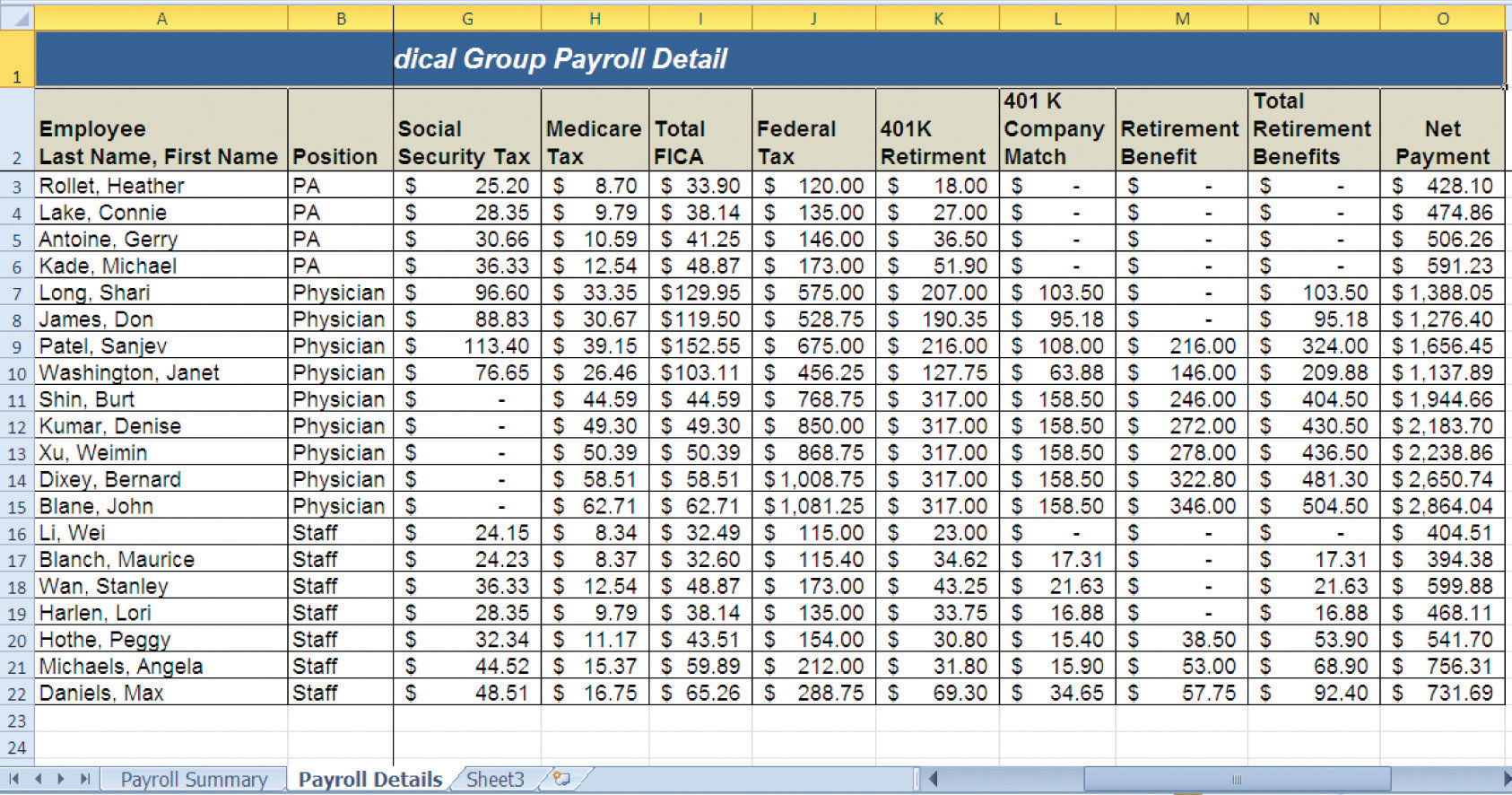
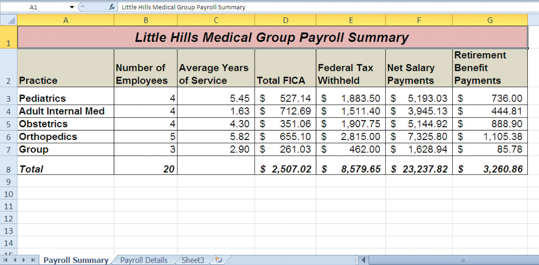
Figure 3.58 Completed CiP Exercise 2 Payroll Summary Worksheet
Integrity Check
Starter File: Chapter 3 IC Exercise 3
Difficulty: Level 3 Difficult
The purpose of this exercise is to analyze a worksheet to determine whether there are any integrity flaws. Read the scenario that follows and then open the Excel workbook related to this exercise. You will find a worksheet in the workbook named AnswerSheet. This worksheet is to be used for any written responses required for this exercise.
Scenario
You recently became the inventory director for a medium-size apparel retail company. The company relies on you to keep a very close watch on the inventory levels for all the items the company sells. Any apparel inventory that is left unsold after the current season will have to be sold at a significant discount. Large excess amounts of inventory can result in drastic profit losses for the company. The company analyzes inventory based on a sell-through rate, which is the weekly unit sales divided by the current inventory units. A sell-through percentage between 12% and 15% is considered normal. At this rate the company will sell all inventory for an item in 6 to 8 weeks. However, a sell-through rate that is outside of this range will require immediate action. An analyst has e-mailed you an inventory status report based on the company’s inventory management guidelines. He explains the following in his e-mail:
- The Status column of the inventory contains a function I put together that tells us where we have issues. The company suggests that we put a “rush priority” on any inventory orders for more than 100 units in a week and for which the sell-through rate is greater than or equal to 20%.
- If the sell-through rate for any item is less than 10%, we have to work with the buyers to see if any incoming orders can be cancelled. The function I created indicates any slow-selling items with a “cancel warning” description.
- Overall, it looks like our biggest problem is that we don’t have enough inventory. In fact, most of the items on the report are showing a “rush priority.” I guess this is a good problem to have.
Assignment
- Look at the Status column (Column E) for the first few items on the inventory report. Does the output of the function created by the analyst make sense given the company’s guidelines for managing inventory? Document your observation in the AnswerSheet worksheet.
- Evaluate the construction of the IF function in the Status column for the first item. Does the function accurately evaluate the Sell Through percentages in Column D? Document your observation in the AnswerSheet worksheet.
- The company suggests that a rush priority be placed on any orders if the unit sales for an item are greater than 100 and the sell-through rate is greater than or equal to 20%. Does the IF function in the Status column accurately account for this condition? Document your observation in the AnswerSheet worksheet.
- Enter a new IF function in the Status column to accurately assess the inventory for each item based on the company’s inventory policies. Make any other adjustments to the worksheet so that it is easy to see all items that require “Rush Priorities” as well “Cancel Warnings.”
Applying Excel Skills
Keeping a Stock Portfolio Current with Web Queries
Starter File: Chapter 3 AES Assignment 1
Difficulty: Level 3 Difficult
The purpose of this exercise is to create a worksheet that tracks a small stock portfolio by utilizing web queries to bring in current price data from the web. The Excel workbook for this assignment contains a small subset of data from the Personal Investment Portfolio that was used to demonstrate the skills in this chapter. Your assignment is to complete the workbook based on the following requirements:
- The Price Data worksheet contains symbols for five stocks. Create a web query for each stock symbol that imports the current stock price from Yahoo! Finance. Set the properties for each web query to retrieve data from the web every 2 minutes. Make sure that the first column of the web query for MSFT begins in cell location A2 on the Price Data worksheet.
- Complete the Current Price column on the Investment Detail worksheet using an HLOOKUP function. Your function should display the “Last Trade” price from the Price Data worksheet for the appropriate stock symbol in Column B in the Investment Detail worksheet.
- Enter formulas in Columns G, H, and I to calculate the Cost of Purchase, Current Value, and Unrealized Gain/Loss. Refer to Table 3.2 "Definitions for Columns A through G of the Investment Detail Worksheet", Table 3.3 "Definitions for Columns H through K of the Investment Detail Worksheet", and Table 3.5 "Definitions for Columns S through X of the Investment Detail Worksheet" earlier in this chapter if needed to create these formulas.
- Show the total Unrealized Gain/Loss for the portfolio in cell I8.
- For any stock, or for the entire portfolio, that is showing an Unrealized Loss in Column I, have Excel automatically change the font color to red and use a bold format.
A Second Look at Federal Income Taxes
Starter File: Chapter 3 AES Assignment 2
Difficulty: Level 3 Difficult
The purpose of this assignment is to revisit the federal payroll tax calculations that were demonstrated in the Careers in Practice: Payroll for a Medical Group exercise. In that exercise, we assumed that if the employee’s weekly income was less than or equal to $1,150, the federal tax was estimated at 20%. For any income over $1,150, the federal tax was estimated at 25%. However, the IRS publishes tables that provide more details as to how federal taxes should be calculated and withheld for weekly payrolls.
The Excel workbook for this assignment contains two worksheets. The Payroll Details worksheet is a subset of the data that was used for the Careers in Practice exercise. The Withholding Table worksheet contains part of an Excel worksheet that was published by the IRS. There are six levels of weekly income in Columns A and B of the worksheet. Columns C and D provide information for calculating the amount of federal tax that should be withheld. For example, if an employee’s weekly salary is $200, you would use Row 3 to calculate the amount of federal tax that should be withheld. This means you would first subtract the value in cell C3 from the weekly salary, which is: 200 − 111.15 = 88.85. Then the result of 88.85 is multiplied by the percentage in cell D3, which is: 88.85 × .10 = 8.885. Therefore, the federal tax that should be withheld for an employee who is paid $200 a week is $8.885. Expressed as a formula, the calculation would be as follows: (200 − 111.15) × .10.
Your assignment is to complete the Federal Tax calculations in Column F of the Payroll Details worksheet. You are required to reference the data in the Withholding Table worksheet such that if the tax rates change in the future (a very common occurrence), your federal tax calculations will automatically be updated. Hint: You will need to use the VLOOKUP function twice in your formula. Follow the example calculation carefully and manually check the output of your formula to determine whether you are producing an accurate result.
The Smart Grade Book
Starter File: Chapter 3 AES Assignment 3
Difficulty: Level 3 Difficult
The Excel workbook for this assignment contains a partially completed grade book for a typical college-level course. The Grade Details worksheet contains a list of hypothetical students who were enrolled in the course as well as the grades they received for each course requirement. Column H contains a formula that calculates the final grade for each student. Table 3.12 "Final Grade Calculation" shows information that was included in the course syllabus that shows students how their final grades will be calculated.
Table 3.12 Final Grade Calculation
| Requirement | Percent of Final Grade |
|---|---|
| Paper 1 | 10 |
| Paper 2 | 10 |
| Class Participation | 15 |
| Quizzes | 10 |
| Midterm Exam | 20 |
| Final Exam | 35 |
| Special Note | A final grade below a 70 will require that this course be repeated for credit. |
The Excel skills demonstrated in this chapter can be used to create a dynamic and “smart” grade book for any academic course. Your assignment is to complete the grade book using several of the Excel skills that you have learned so far. Open the Excel workbook for this assignment and complete the grade book based on the following requirements:
- It is very important to make sure a student’s grade is accurately calculated. One area that must be checked often when calculating final grades is the percentages assigned to each requirement in the course. One way to do this is to see if the percentages add up to 100%. Use an IF function in the merged cells H2 and I2 on the Grade Details worksheet to determine if the percentages in the range B2:G2 add up to 100%. If the percentages do not add up to 100%, show the phrase “Percentages do not equal 100%.” Otherwise, leave the cell blank (use two quotation marks: “”). Use the results of your IF function to make any necessary adjustments to the grade book (refer to Table 3.12 "Final Grade Calculation" as needed).
- Calculate class averages in Row 29 for each course requirement as well as the final grades in Columns B through H.
- Use a VLOOKUP function to display the appropriate letter grade for each student in Column I. The Grade Table worksheet contains data that show how the letter grades should be assigned for the numeric grades.
- Complete the Class Grade Distribution in the range I32:I43 on the Grade Details worksheet. The purpose of this area is to show how many students received the grades listed in the range H32:H43. For example, how many students receive an A, A−, and so on. Include a percent of total for each grade. Hint: This can be accomplished using the COUNTIF function if you successfully complete the VLOOKUP function in step 3. If you are unable to complete step 3, you can still complete this step using the COUNTIFS function.
- Add any formatting enhancements to the Grade Details worksheet that would make the worksheet easier to read and use. Consider the “Special Note” in Table 3.12 "Final Grade Calculation".
Chapter Skills Test
Starter File: Chapter 3 Skills Test
Difficulty: Level 2 Moderate
Answer the following questions by executing the skills on the starter file required for this test. Answer each question in the order in which it appears. If you do not know the answer, skip to the next question. Open the starter file before you begin this test.
- Set the Freeze Panes command so that Rows 1 and 2 and Columns A and B are locked in place while scrolling through the Investment Detail worksheet.
- In the Investment Detail worksheet, enter an IF function into cell I3. The output of the function should be the word Gain if the Current Investment Value in cell H3 is greater than the Cost of Purchase in cell G3. Otherwise, the output of the function should be the words No Gain.
- Copy the IF function in cell I3 and paste it into the range I4:I17 using the Paste Formulas command.
- In the Investment Detail worksheet, enter a nested IF function into cell F3. If the Dividend/Yield value in cell E3 is less than 2%, show the word Low. If the Dividend/Yield value in cell E3 is greater than or equal to 5%, show the word High. Otherwise, show the word Moderate.
- Copy the IF function in cell F3 and paste it into the range F4:F17 using the Paste Formulas command.
- On the Investment Detail worksheet in cell O3, use the OR function within an IF function to evaluate the Current vs. Target value. If the Current vs. Target value in cell N3 is greater than 2% or less than −2%, show the word REBAL. Otherwise, show the word OK.
- Copy the IF function in cell O3 and paste it into the range O4:O17 using the Paste Formulas command.
- On the Investment Detail worksheet in cell P3, use the AND function within an IF function to evaluate the Current vs. Target value and the Unrealized Gain/Loss value. If the Current vs. Target value in cell N3 is greater than 2% and if the Unrealized Gain/Loss value in cell J3 is greater than 0, show the word BUY. Otherwise, show the word HOLD.
- Copy the IF function in cell P3 and paste it into the range P4:P17 using the Paste Formulas command.
- On the Investment Detail worksheet, apply a conditional format to the range Q3:Q17. If the Months Owned is less than 12, change the font color to red. Otherwise, the font color should remain black.
- On the Investment Detail worksheet, enter a VLOOKUP function in cell D3 that displays the Growth Last Year for the symbol in cell B3. The growth last year for all investments can be found in Column E on the Investment List worksheet. Your function should look for an exact match to the lookup value. Consider that this function will be copied and pasted into the range D4:D17 when defining the arguments.
- On the Investment Detail worksheet, format the range D3:D17 to a percentage with two decimal places. Then copy the VLOOKUP function in cell D3 and paste it into the range D4:D17 using the Paste Formulas command.
- On the Portfolio Summary worksheet, use the COUNTIF function in cell B3 to count the number of investments that match the investment type in cell A3. The function should look for and count the number of investment types in the range A3:A17 on the Investment Detail worksheet. Consider that this function will be copied and pasted into the range B4:B6 when defining the arguments.
- Copy the COUNTIF function in cell B3 and paste it into the range B4:B6 using the Paste Formulas command.
- On the Portfolio Summary worksheet, use the AVERAGEIF function in cell C3 to calculate the average Dividend/Yield for the investment type in cell A3. The function should calculate the average using the data in the range E3:E17 on the Investment Detail worksheet. The function should look for a match to the investment type in the range A3:A17 on the Investment Detail worksheet. Consider that this function will be copied and pasted into the range C4:C6 when defining the arguments.
- Copy the AVERAGEIF function in cell C3 and paste it into the range C4:C6 using the Paste Formulas command.
- On the Portfolio Summary worksheet, use the SUMIF function in cell D3 to calculate the Percent of Portfolio for the investment type in cell A3. The function should calculate the sum using the data in the range L3:L17 on the Investment Detail worksheet. The function should look for a match to the investment type in the range A3:A17 on the Investment Detail worksheet. Consider that this function will be copied and pasted into the range D4:D6 when defining the arguments.
- Copy the SUMIF function in cell D3 and paste it into the range D4:D6 using the Paste Formulas command.
- On the Portfolio Summary worksheet, use the HLOOKUP function to display the Portfolio Target in cell E3. The function should look for the Investment Type in cell A3 in Row 2 of the Portfolio Targets worksheet. The function should display the percentage in the Moderate row (Row 5) for each investment type. The function should look for an exact match to the lookup value. Consider that this function will be copied and pasted into the range E4:E6 when defining the arguments.
- Copy the HLOOKUP function in cell E3 and paste it into the range E4:E6 using the Paste Formulas command.
- On the Portfolio Summary worksheet, use the COUNTIFS function in cell B10 to count the number of investments that match the investment type in cell A10 and have an unrealized gain that is greater than or equal to 20%. The function should look for and count the investment types in the range A3:A17 on the Investment Detail worksheet where the Percent Gain/Loss in the range K3:K17 is greater than or equal to 20%. Consider that this function will be copied and pasted into the range B11:B13 when defining the arguments.
- Copy the COUNTIFS function in cell B10 and paste it into the range B11:B13 using the Paste Formulas command.
- On the Portfolio Summary worksheet, use the SUMIFS function in cell C10 to sum the Total Unrealized Gain for the investment type in cell A10 where the unrealized gain is greater than or equal to 20%. The function should calculate the sum using the data in the range J3:J17 on the Investment Detail worksheet. The function should look for a match to the investment type in the range A3:A17 on the Investment Detail worksheet where the Percent Gain/Loss in the range K3:K17 is greater than or equal to 20%. Consider that this function will be copied and pasted into the range C11:C13 when defining the arguments.
- Copy the SUMIFS function in cell C10 and paste it into the range C11:C13 using the Paste Formulas command.
- On the Portfolio Summary worksheet, use the AVERAGEIFS function in cell D10 to calculate the average Dividend/Yield for the investment type in cell A10 where the unrealized gain is greater than or equal to 20%. The function should calculate the average using the data in the range E3:E17 on the Investment Detail worksheet. The function should look for a match to the investment type in the range A3:A17 on the Investment Detail worksheet where the Percent Gain/Loss in the range K3:K17 is greater than or equal to 20%. Consider that this function will be copied and pasted into the range D11:D13 when defining the arguments.
- Copy the AVERAGEIFS function in cell D10 and paste it into the range D11:D13 using the Paste Formulas command.
- Save the workbook by adding your name in front of the current workbook name (i.e., “your name Chapter 3 Skills Test”).
- Close the workbook and Excel.