This is “Fundamental Skills”, chapter 1 from the book Using Microsoft Excel (v. 1.0). For details on it (including licensing), click here.
For more information on the source of this book, or why it is available for free, please see the project's home page. You can browse or download additional books there. To download a .zip file containing this book to use offline, simply click here.


Chapter 1 Fundamental Skills
Microsoft® Excel® is a tool that can be used in virtually all careers and is valuable in both professional and personal settings. Whether you need to keep track of medications in inventory for a hospital or create a financial plan for your retirement, Excel enables you to do these activities efficiently and accurately. This chapter introduces the fundamental skills necessary to get you started in using Excel. You will find that just a few skills can make you very productive in a short period of time.
1.1 An Overview of Microsoft® Excel®
Learning Objectives
- Examine the value of using Excel to make decisions.
- Learn how to start Excel.
- Become familiar with the Excel workbook.
- Understand how to navigate worksheets.
- Examine the Excel Ribbon.
- Become familiar with the Quick Access Toolbar.
- Examine the right-click menu options.
- Become familiar with the commands in the File tab.
- Learn how to save workbooks.
- Save workbooks in the Excel 97-2003 file type.
- Examine the Status Bar.
- Become familiar with the features in the Excel Help window.
Microsoft® Office contains a variety of tools that help people accomplish many personal and professional objectives. Microsoft Excel is perhaps the most versatile and widely used of all the Office applications. No matter which career path you choose, you will likely need to use Excel to accomplish your professional objectives, some of which may occur daily. This chapter provides an overview of the Excel application along with an orientation for accessing the commands and features of an Excel workbook.
Making Decisions with Excel
Follow-along file: Not needed for this skill
Taking a very simple view, Excel is a tool that allows you to enter quantitative data into an electronic spreadsheet to apply one or many mathematical computations. These computations ultimately convert that quantitative data into information. The information produced in Excel can be used to make decisions in both professional and personal contexts. For example, employees can use Excel to determine how much inventory to buy for a clothing retailer, how much medication to administer to a patient, or how much money to spend to stay within a budget. With respect to personal decisions, you can use Excel to determine how much money you can spend on a house, how much you can spend on car lease payments, or how much you need to save to reach your retirement goals. We will demonstrate how you can use Excel to make these decisions and many more throughout this text.
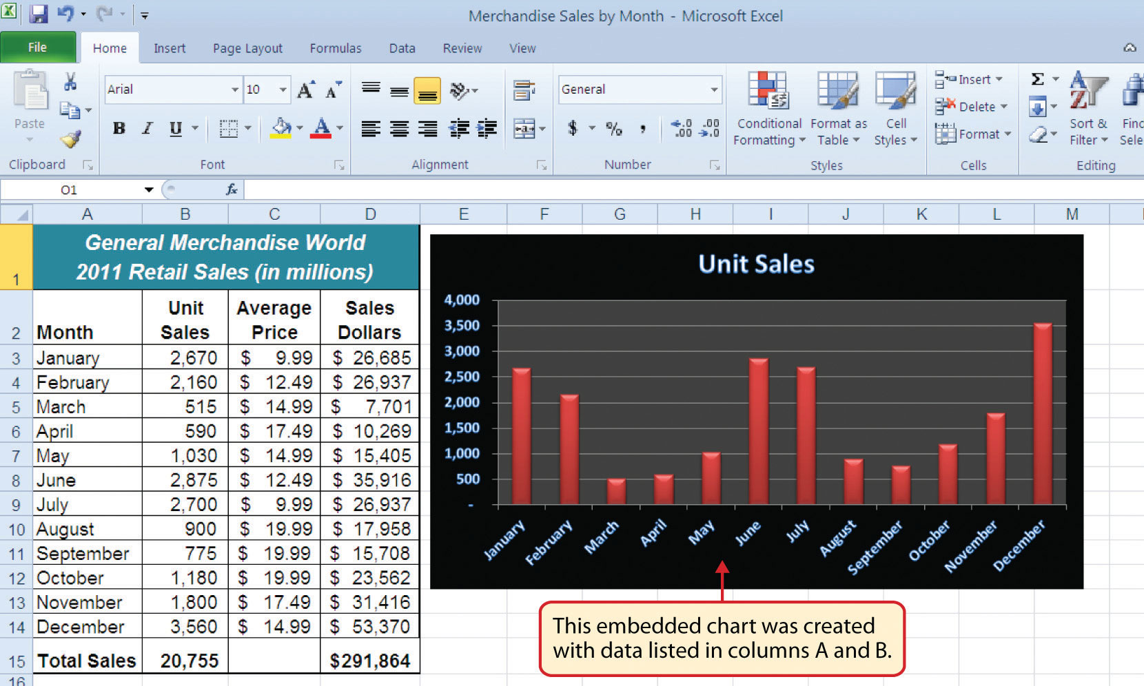
Figure 1.1 "Example of an Excel Worksheet with Embedded Chart" shows a completed Excel worksheet that will be constructed in this chapter. The information shown in this worksheet is top-line sales data for a hypothetical merchandise retail company. The worksheet data can help this retailer determine the number of salespeople needed for each month, how much inventory is needed to satisfy sales, and what types of products should be purchased. Notice that the embedded chart makes it very easy to see which months have the highest unit sales.
Figure 1.1 Example of an Excel Worksheet with Embedded Chart
Starting Excel
Follow-along file: Not needed for this skill
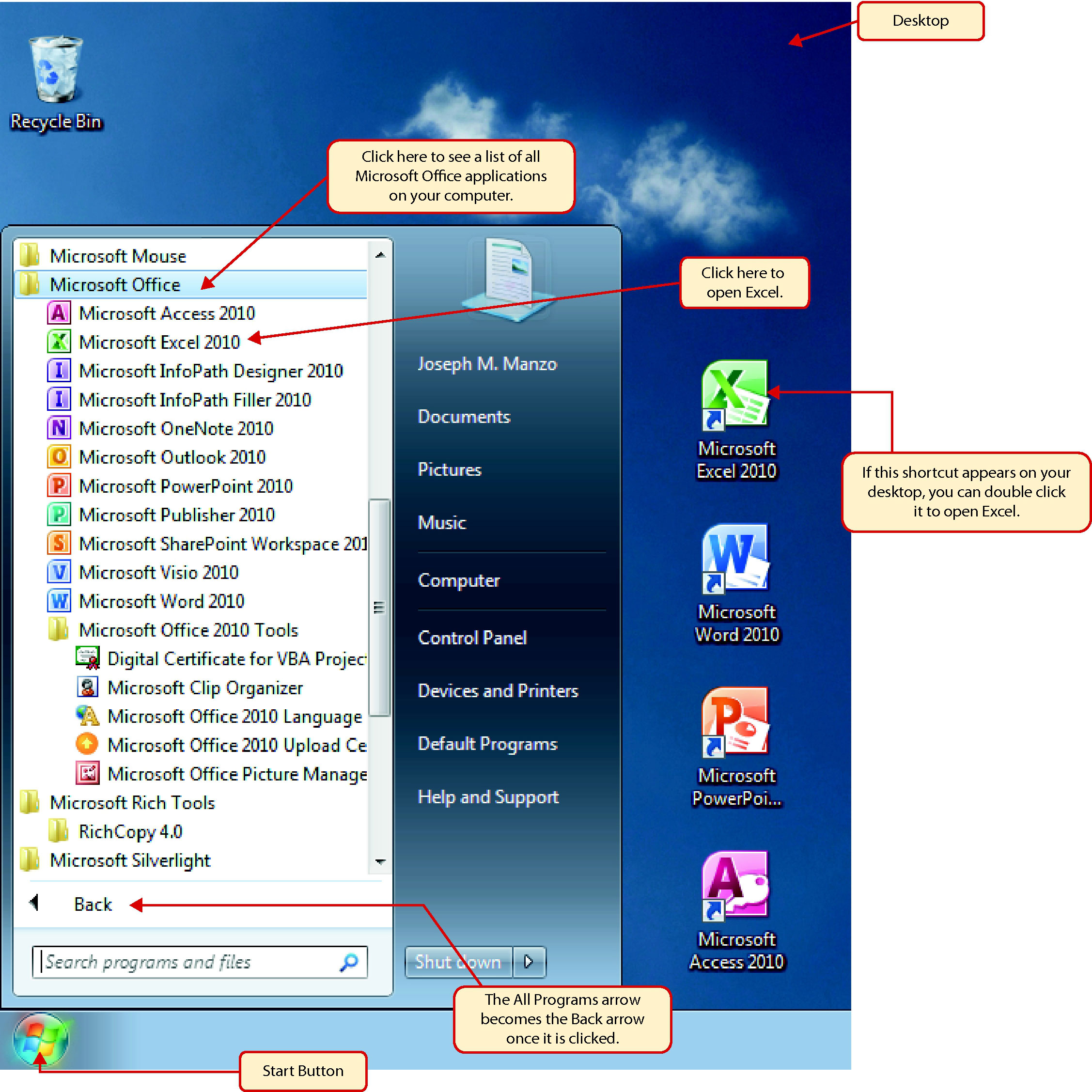
The following steps will guide you in starting the Excel application. Note that these steps along with Figure 1.2 "Start Menu" relate to the Windows 7 operating system, which is very similar to the Windows Vista operating system.
- Click the Start button on the lower left corner of your computer screen.
- Click the All Programs arrow at the bottom left of the Start menu.
- Click the Microsoft Office folder on the Start menu. This will open the list of Microsoft Office applications.
- Click the Microsoft Excel 2010 option. This will start the Excel application.
Figure 1.2 Start Menu
The Excel Workbook
Follow-along file: Not needed for this skill
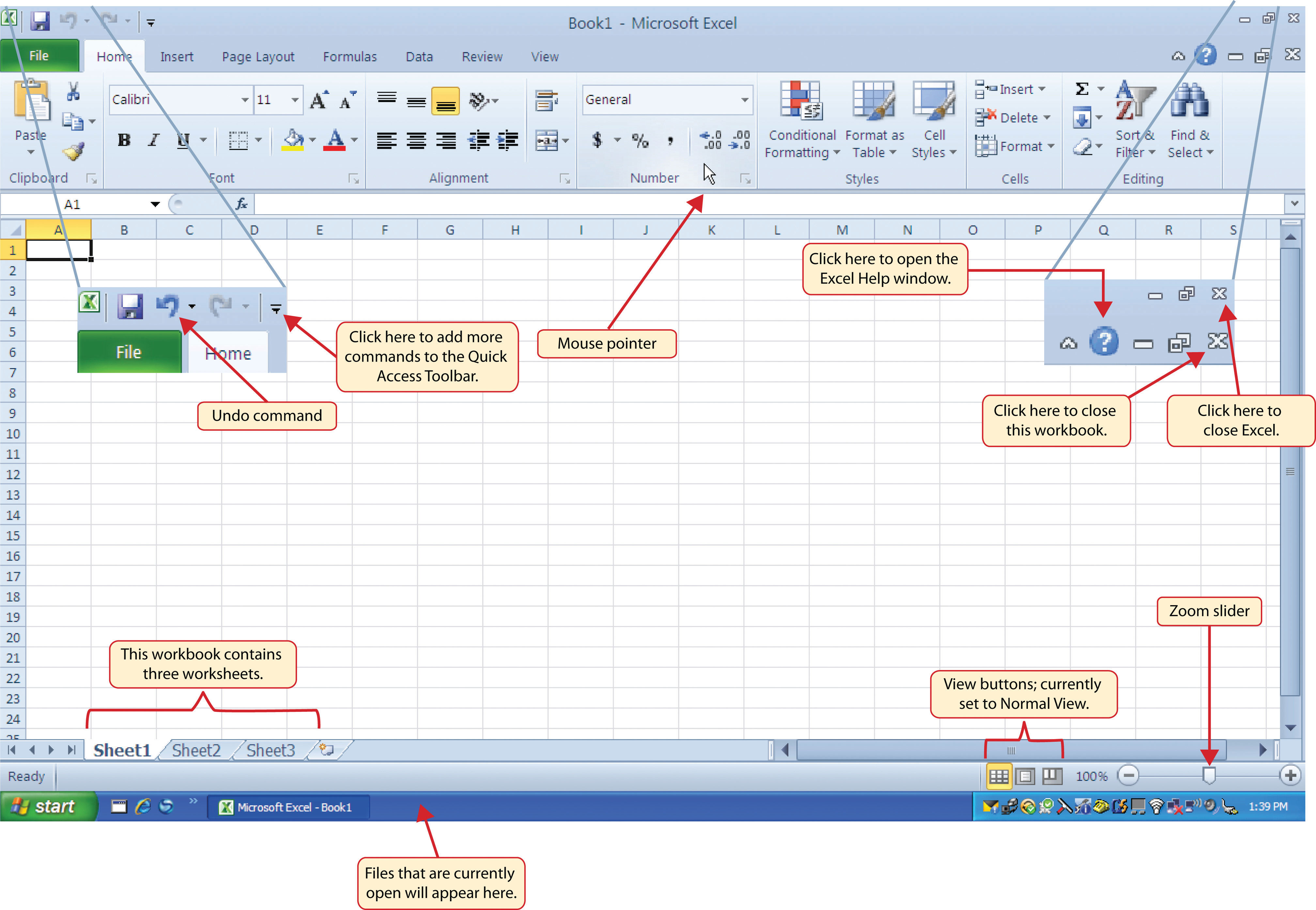
Once Excel is started, a blank workbook will open on your screen. A workbookAn Excel file that contains one or more worksheets. is an Excel file that contains one or more worksheetsMay also be referred to as a spreadsheet and contains rectangles called cells for entering numeric and nonnumeric data. (sometimes referred to as spreadsheets). Excel will assign a file name to the workbook, such as Book1, Book2, Book3, and so on, depending on how many new workbooks are opened. Figure 1.3 "Blank Workbook" shows a blank workbook after starting Excel.
Figure 1.3 Blank Workbook
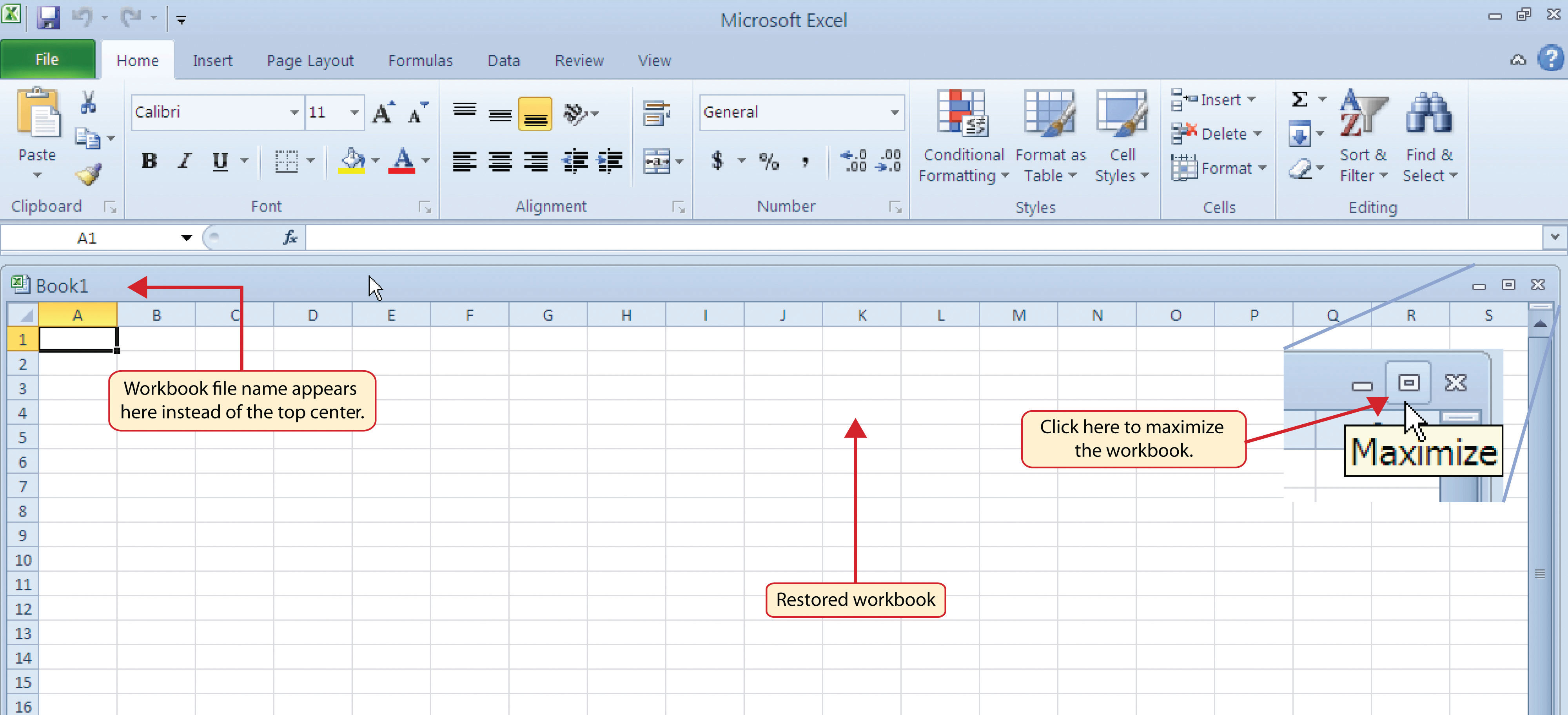
Your workbook should already be maximized (or shown at full size) once Excel is started, as shown in Figure 1.3 "Blank Workbook". However, if your screen looks like Figure 1.4 "Restored Worksheet" after starting Excel, you should click the Maximize button, as shown in the figure.
Figure 1.4 Restored Worksheet
Navigating Worksheets
Follow-along file: Not needed for this skill
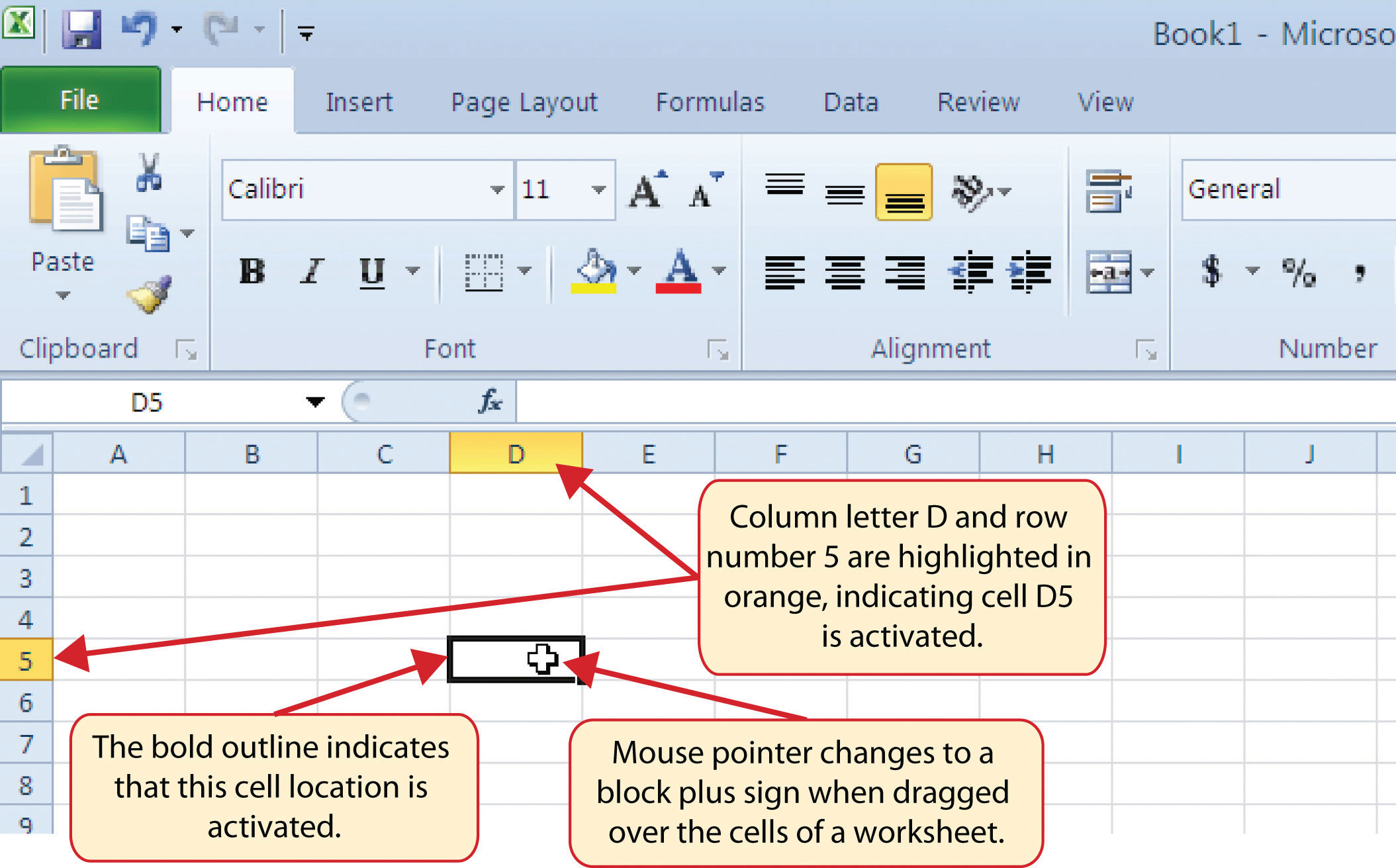
Data are entered and managed in an Excel worksheet. The worksheet contains several rectangles called cells for entering numeric and nonnumeric data. Each cellA specific location on a worksheet where data are entered and stored. in an Excel worksheet contains an address, which is defined by a column letter followed by a row number. For example, the cell that is currently activated in Figure 1.4 "Restored Worksheet" is A1. This would be referred to as cell locationA column letter followed by a row number used to identify specific cells on a worksheet. A1 or cell referenceWhen cell locations are used in formulas, Excel will reference the data that is entered into the cell. The cell reference is the cell location address. A1. The following steps explain how you can navigate in an Excel worksheet:
- Place your mouse pointer over cell D5 and left click.
-
Check to make sure column letter D and row number 5 are highlighted in orange, as shown in Figure 1.5 "Activating a Cell Location".
Figure 1.5 Activating a Cell Location
- Move the mouse pointer to cell A1.
- Click and hold the left mouse button and drag the mouse pointer back to cell D5.
-
Release the left mouse button. You should see several cells highlighted, as shown in Figure 1.6 "Highlighting a Range of Cells". This is referred to as a cell rangeAny group of contiguous cell locations; a cell range is noted as two cell locations separated by a colon. and is documented as follows: A1:D5. Any two cell locations separated by a colon are known as a cell range. The first cell is the top left corner of the range, and the second cell is the lower right corner of the range.
Figure 1.6 Highlighting a Range of Cells
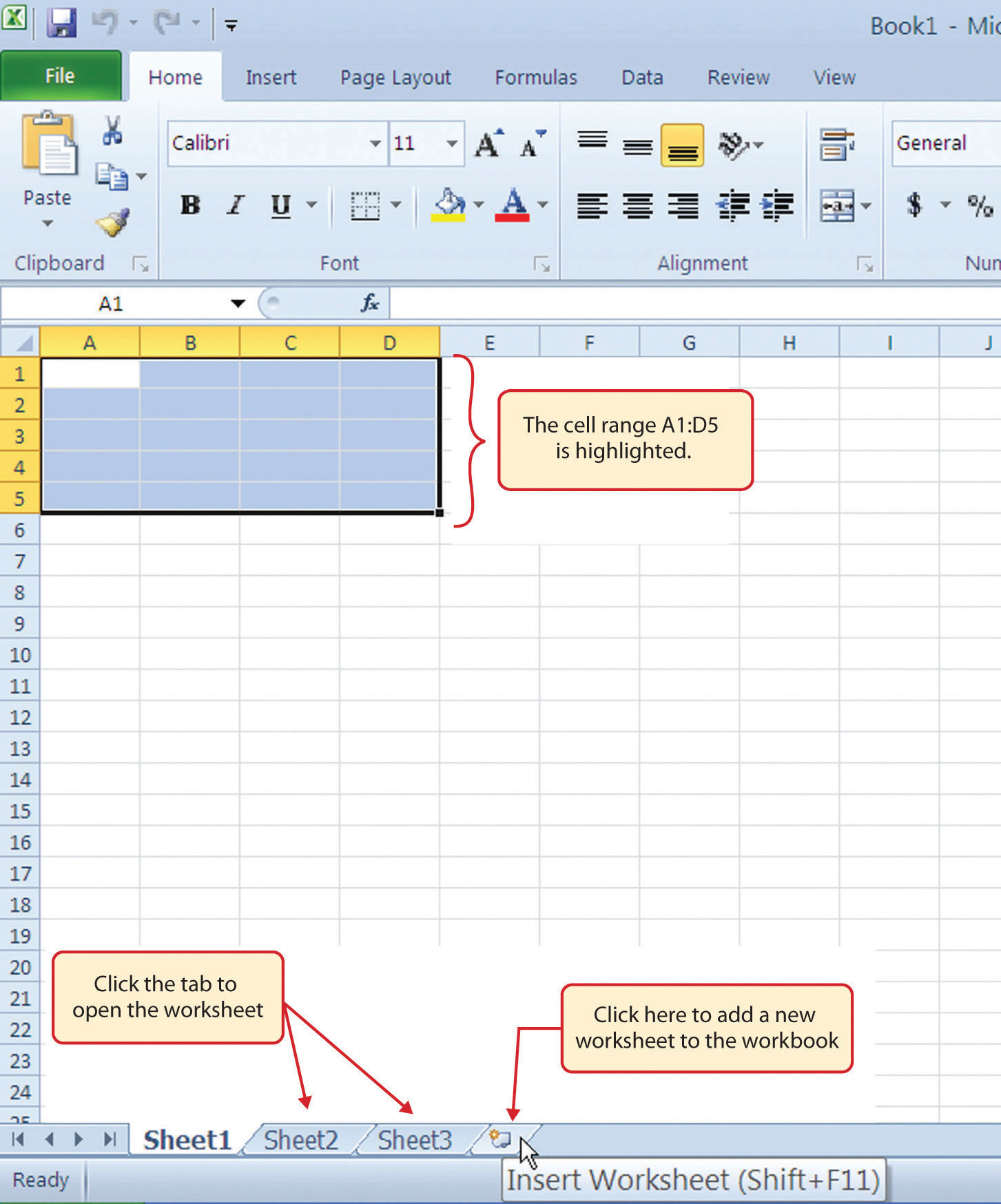
- Click the Sheet3 worksheet tab at the bottom of the worksheet. This is how you open a worksheet within a workbook.
- Click the Sheet1 worksheet tab at the bottom of the worksheet to return to the worksheet shown in Figure 1.6 "Highlighting a Range of Cells".
Mouseless Commands
Basic Worksheet Navigation
- Use the arrow keys on your keyboard to activate cells on the worksheet.
- Hold the SHIFT key and press the arrow keys on your keyboard to highlight a range of cells in a worksheet.
- Hold the CTRL key while pressing the PAGE DOWN or PAGE UP keys to open other worksheets in a workbook.
The Excel Ribbon
Follow-along file: Not needed for this skill
Excel’s features and commands are found in the RibbonThe upper area of the Excel screen that contains several tabs running across the top. Each tab provides access to a different set of Excel commands., which is the upper area of the Excel screen that contains several tabs running across the top. Each tab provides access to a different set of Excel commands. Figure 1.7 "Ribbon for Excel" shows the commands available in the Home tab of the Ribbon. Table 1.1 "Command Overview for Each Tab of the Ribbon" provides an overview of the commands that are found in each tab of the Ribbon.
Figure 1.7 Ribbon for Excel
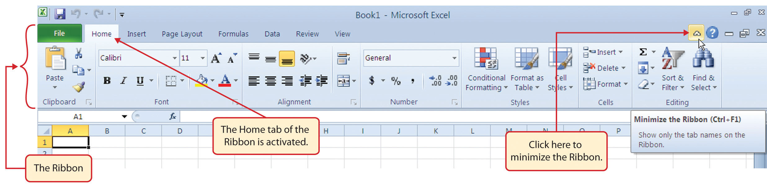
Table 1.1 Command Overview for Each Tab of the Ribbon
| Tab Name | Description of Commands |
|---|---|
| File | Also known as the Backstage view of the Excel workbook. Contains all commands for opening, closing, saving, and creating new Excel workbooks. Includes print commands, document properties, e-mailing options, and help features. The default settings and options are also found in this tab. |
| Home | Contains the most frequently used Excel commands. Formatting commands are found in this tab along with commands for cutting, copying, pasting, and for inserting and deleting rows and columns. |
| Insert | Used to insert objects such as charts, pictures, shapes, PivotTables, Internet links, symbols, or text boxes. |
| Page Layout | Contains commands used to prepare a worksheet for printing. Also includes commands used to show and print the gridlines on a worksheet. |
| Formulas | Includes commands for adding mathematical functions to a worksheet. Also contains tools for auditing mathematical formulas. |
| Data | Used when working with external data sources such as Microsoft® Access®, text files, or the Internet. Also contains sorting commands and access to scenario tools. |
| Review | Includes Spelling and Track Changes features. Also contains protection features to password protect worksheets or workbooks. |
| View | Used to adjust the visual appearance of a workbook. Common commands include the Zoom and Page Layout view. |
The Ribbon shown in Figure 1.7 "Ribbon for Excel" is full, or maximized. The benefit of having a full Ribbon is that the commands are always visible while you are developing a worksheet. However, depending on the screen dimensions of your computer, you may find that the Ribbon takes up too much vertical space on your worksheet. If this is the case, you can minimize the Ribbon by clicking the button shown in Figure 1.7 "Ribbon for Excel". When minimized, the Ribbon will show only the tabs and not the command buttons. When you click on a tab, the command buttons will appear until you select a command or click anywhere on your worksheet.
Mouseless Commands
Minimizing or Maximizing the Ribbon
- Hold down the CTRL key and press the F1 key.
- Hold down the CTRL key and press the F1 key again to maximize the Ribbon.
Quick Access Toolbar and Right-Click Menu
Follow-along file: Not needed for this skill
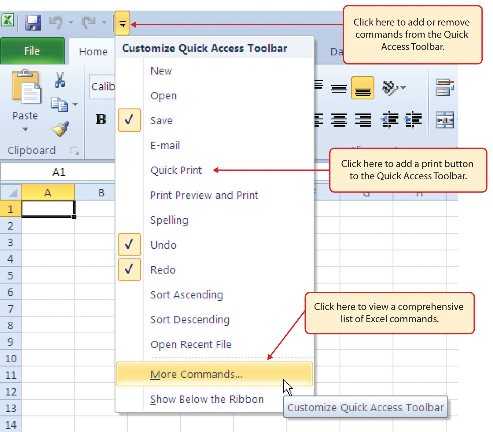
The Quick Access ToolbarLocated at the upper-left side of the Excel screen above the Ribbon, this toolbar provides access to the most frequently used commands, such as Save and Undo. is found at the upper left side of the Excel screen above the Ribbon, as shown in Figure 1.3 "Blank Workbook". This area provides access to the most frequently used commands, such as Save and Undo. You also can customize the Quick Access Toolbar by adding commands that you use on a regular basis. By placing these commands in the Quick Access Toolbar, you do not have to navigate through the Ribbon to find them. To customize the Quick Access Toolbar, click the down arrow as shown in Figure 1.8 "Customizing the Quick Access Toolbar". This will open a menu of commands that you can add to the Quick Access Toolbar. If you do not see the command you are looking for on the list, select the More Commands option.
Figure 1.8 Customizing the Quick Access Toolbar
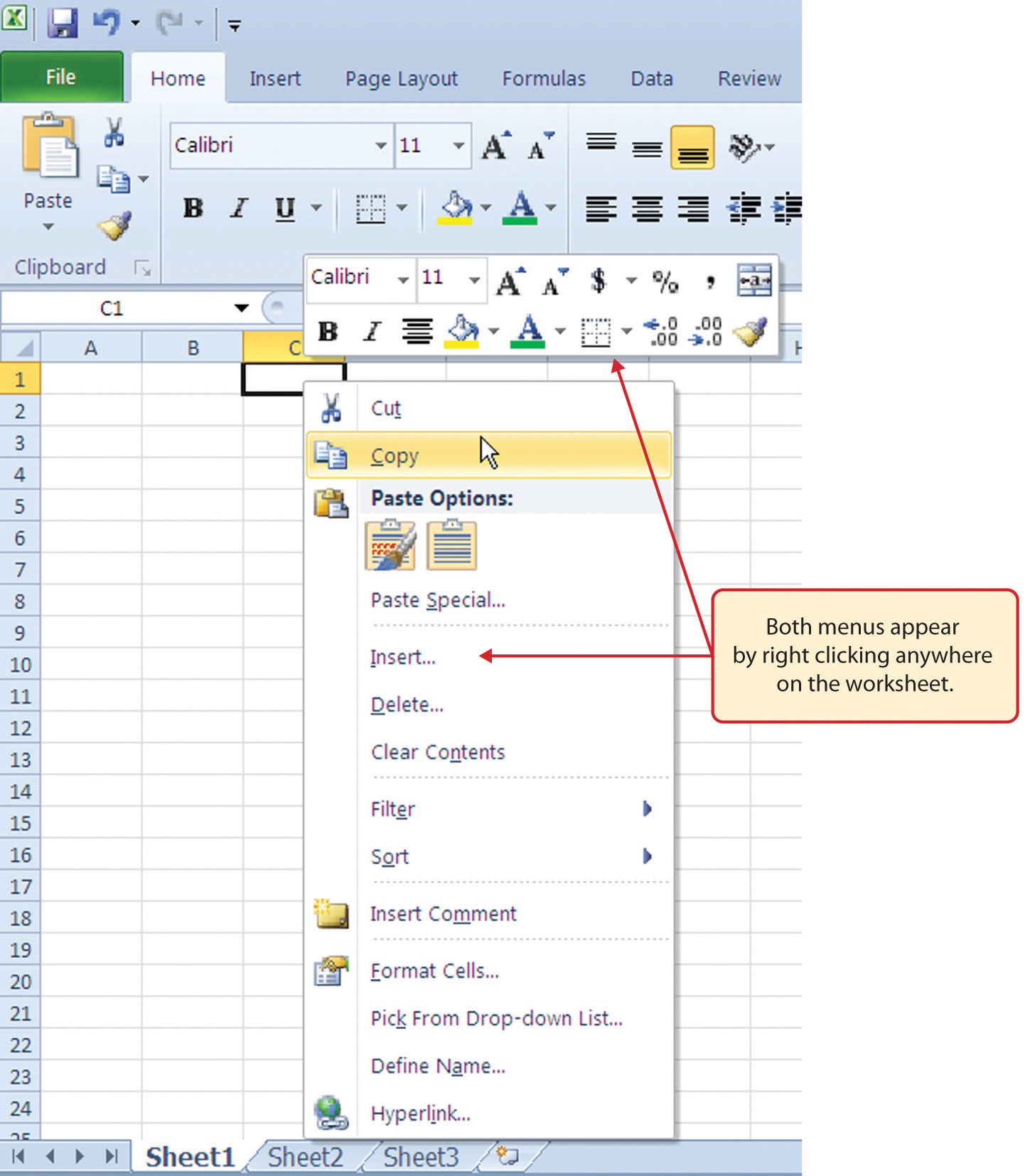
In addition to the Ribbon and Quick Access Toolbar, you can also access commands by right clicking anywhere on the worksheet. Figure 1.9 "Right-Click Menu" shows an example of the commands available in the right-click menu.
Figure 1.9 Right-Click Menu
The File Tab
Follow-along file: Not needed for this skill
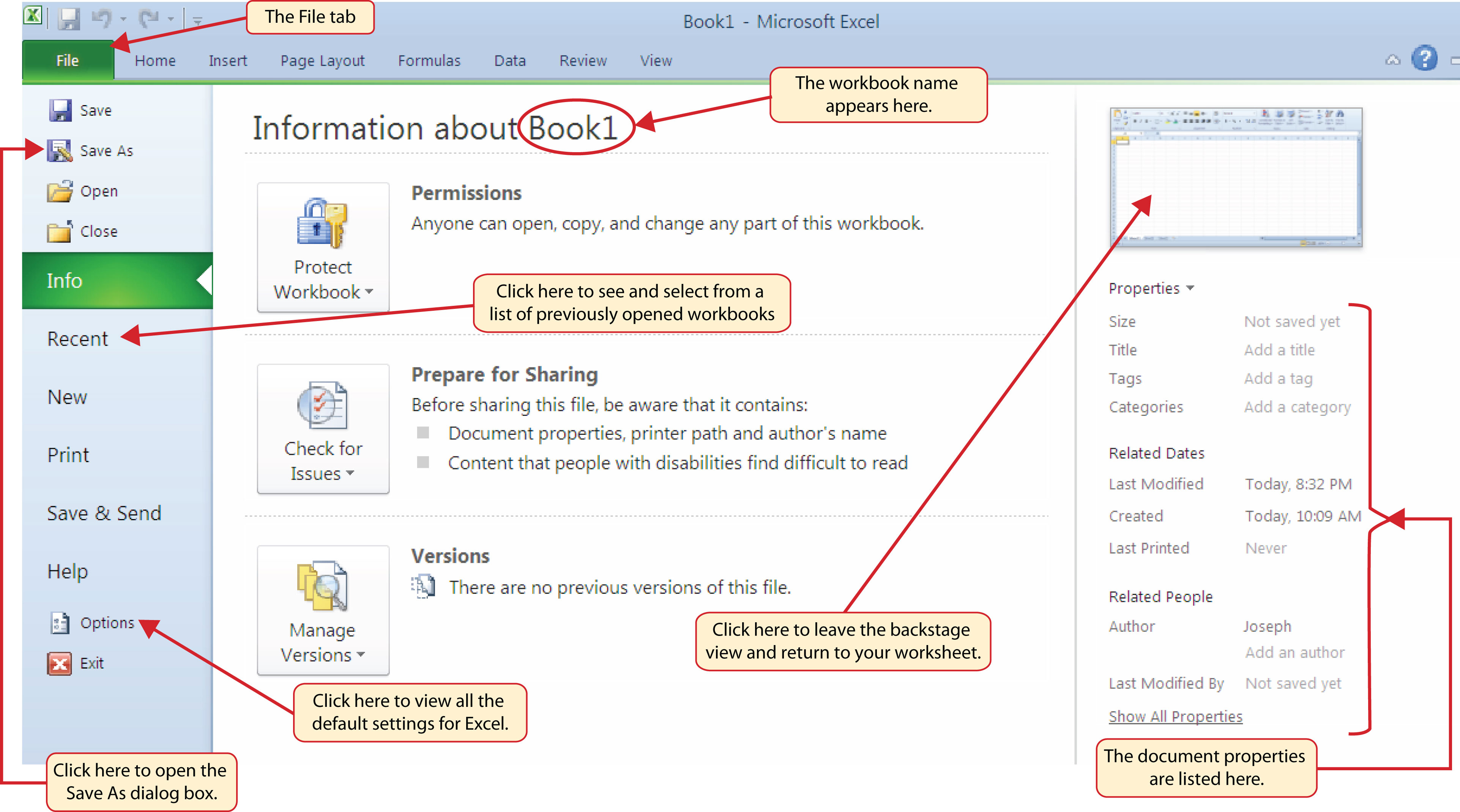
If you have used Office 2007, you may have noticed that the Office button has disappeared in the 2010 version. It has been replaced with the File tab on the far left side of the Ribbon. The File tab is also known as the Backstage viewThis view, which is opened through the File tab on the Ribbon, contains a variety of features and commands related to the workbook that is currently open. of the workbook. It contains a variety of features and commands related to the workbook that is currently open, new workbooks, or workbooks stored in other locations on your computer or network. Figure 1.10 "File Tab or Backstage View of a Workbook" shows the options available in the File tab or Backstage view. To leave the Backstage view and return to the worksheet, click any tab on the Ribbon or click the image of the worksheet on the right side of the window. You must click the Info button (highlighted in green in Figure 1.10 "File Tab or Backstage View of a Workbook") to see the image of your worksheet on the right side of the window.
Figure 1.10 File Tab or Backstage View of a Workbook
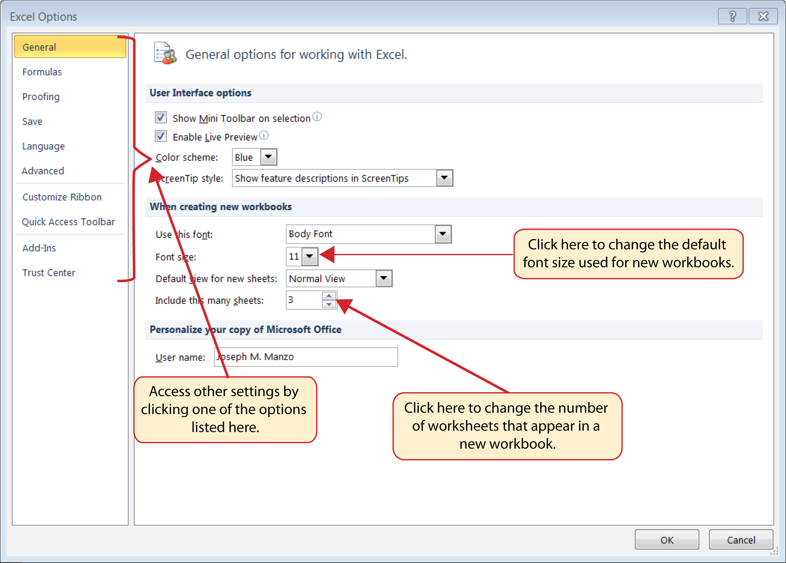
Included in the File tab are the default settings for the Excel application that can be accessed and modified by clicking the Options button. Figure 1.11 "Excel Options Window" shows the Excel Options window, which gives you access to settings such as the default font style, font size, and the number of worksheets that appear in new workbooks.
Figure 1.11 Excel Options Window
Saving Workbooks (Save As)
Follow-along file: Not needed for this skill
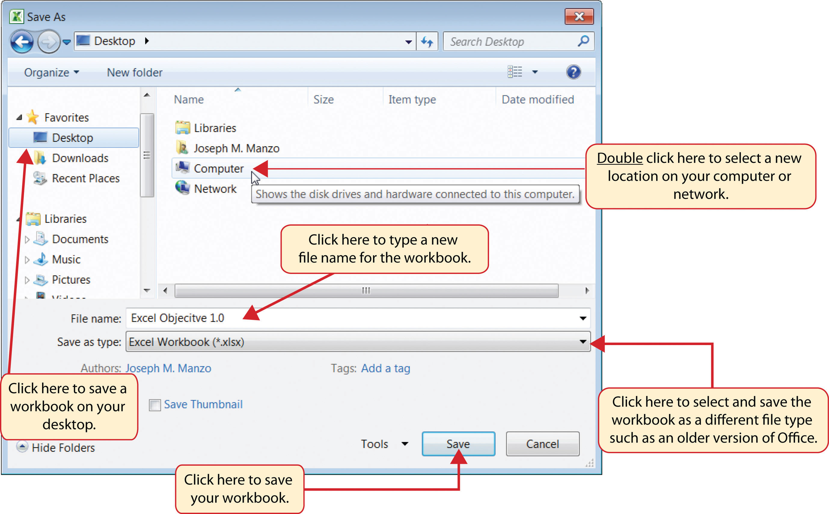
Once you create a new workbook, you will need to change the file name and choose a location on your computer or network to save it. The following steps explain how to save a new workbook and assign it a file name. It is important to remember where you save this workbook on your computer or network as you will be using this file in the Section 1.2 "Entering, Editing, and Managing Data" to construct the workbook shown in Figure 1.1 "Example of an Excel Worksheet with Embedded Chart".
- If you have not done so already, start Excel. A blank workbook should appear on your screen. Check to make sure the workbook is maximized (see Figure 1.4 "Restored Worksheet").
- Click the File tab.
- Click the Save As button in the upper left side of the Backstage view window, as shown in Figure 1.10 "File Tab or Backstage View of a Workbook". This will open the Save As dialog box.
- Click in the File Name box at the bottom of the Save As dialog box.
- Use the BACKSPACE key to remove the current file name of the workbook.
- Type the file name: Excel Objective 1.0.
- Click the Desktop button on the left side of the Save As dialog box if you wish to save this file on your desktop. If you want to save this workbook in a different location on your computer or network, double click the Computer option, as shown in Figure 1.12 "Save As Dialog Box", and select your preferred location.
- Click the Save button on the lower right side of the Save As dialog box.
Figure 1.12 Save As Dialog Box
Mouseless Commands
Save As
- Press the F12 key and use the tab and arrow keys to navigate around the Save As dialog box. Use the ENTER key to make a selection.
- Or press the ALT key on your keyboard. You will see letters and numbers, called Key Tips, appear on the Ribbon. Press the F key on your keyboard for the File tab and then the A key. This will open the Save As dialog box.
Skill Refresher: Saving Workbooks (Save As)
- Click the File tab on the Ribbon.
- Click the Save As option.
- Select a location on your PC or network.
- Click in the File name box and type a new file name if needed.
- Click the down arrow next to the “Save as type” box and select the appropriate file type if needed.
- Click the Save button.
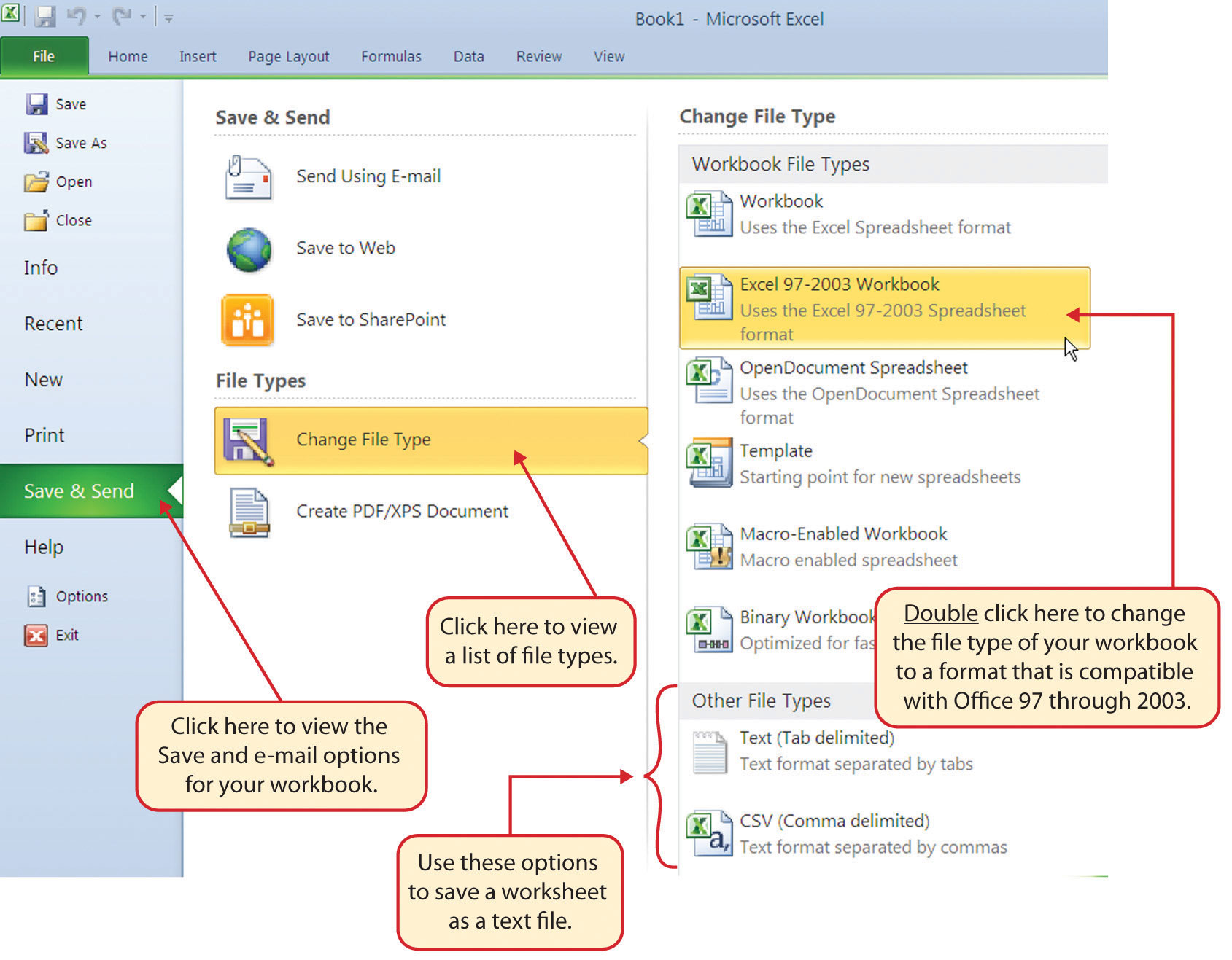
Excel 97-2003 File Type
Follow-along file: Open a blank workbook.
If you are working with someone who is using a version of Microsoft Office that is older than Office 2007, you will have to save your workbook under the Excel 97-2003 Workbook format. A person who is running Office 2003 will not be able to open workbooks that are saved under the Office 2010 or Office 2007 file types. You can save a workbook as an Excel 97-2003 file type by clicking the down arrow next to the “Save as type” box in the Save As dialog box (see Figure 1.12 "Save As Dialog Box").
You can also change the file type of your workbook by using the File tab on the Ribbon. The following steps explain this method:
- Open the workbook you wish to convert to the Excel 97-2003 file type.
- Click the File tab on the Ribbon.
- Click the Save & Send button on the left side of the Backstage view.
- Click the Change File Type button.
- Double click the Excel 97-2003 Workbook option on the right side of the Backstage view. This will open up the Save As dialog box and set the file type box to Excel 97-2003 Workbook (see Figure 1.13 "Changing the File Type of a Workbook").
- Check to make sure the Save As dialog box is set to the location where you want to save your workbook.
- Click the Save button at the bottom of the Save As dialog box.
Figure 1.13 Changing the File Type of a Workbook
Why?
No Office 2007 File Type
Workbooks that are created in Office 2010 are automatically compatible with Office 2007. A person who is running Office 2007 will be able to open, edit, and save workbooks created in Office 2010.
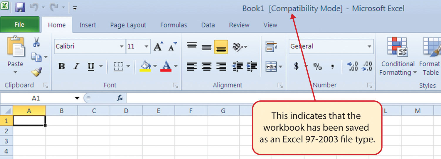
When you convert an existing workbook created in Office 2010 to the Excel 97-2003 file type, you may not notice any changes on the workbook itself. If you are using a feature or format that is not compatible with Office 97-2003, a warning will appear upon saving the file. You may want to remove these features and formats before sending the workbook to a person who is running an older version of Office. When you open a file that is saved in the Excel 97-2003 format, you will see the Compatibility Mode indicator next to the workbook name, as shown in Figure 1.14 "Workbook That Has Been Saved in Excel 97-2003 Format".
Figure 1.14 Workbook That Has Been Saved in Excel 97-2003 Format
The Status Bar
Follow-along file: Continue with a blank workbook or open a new one.
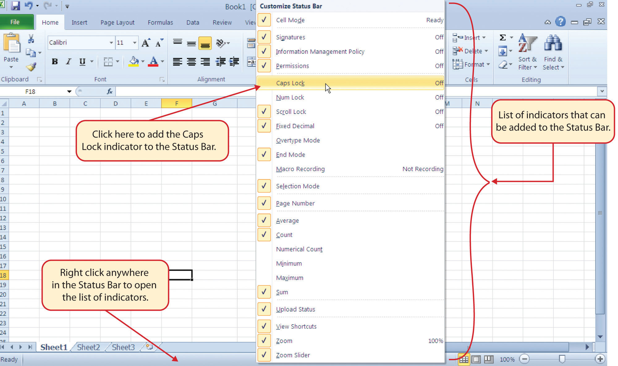
The Status BarLocated below the worksheet tabs on the Excel screen, it displays a variety of information, such as the status of certain keys on your keyboard (e.g., CAPS LOCK), the available views for a workbook, the magnification of the screen, or mathematical functions that can be performed when data are highlighted on a worksheet. is located below the worksheet tabs on the Excel screen (see Figure 1.15 "Customizing the Status Bar"). It displays a variety of information, such as the status of certain keys on your keyboard (e.g., CAPS LOCK), the available views for a workbook, the magnification of the screen, and mathematical functions that can be performed when data are highlighted on a worksheet. You can customize the Status Bar as follows:
- Place the mouse pointer over any area of the Status Bar and right click (see Figure 1.15 "Customizing the Status Bar").
- Select the Caps Lock option from the menu (see Figure 1.15 "Customizing the Status Bar").
- Press the CAPS LOCK key on your keyboard. You will see the Caps Lock indicator on the lower right side of the Status Bar.
- Press the CAPS LOCK key again. The indicator on the Status Bar goes away.
Figure 1.15 Customizing the Status Bar
Excel Help
Follow-along file: Continue with a blank workbook or open a new one.
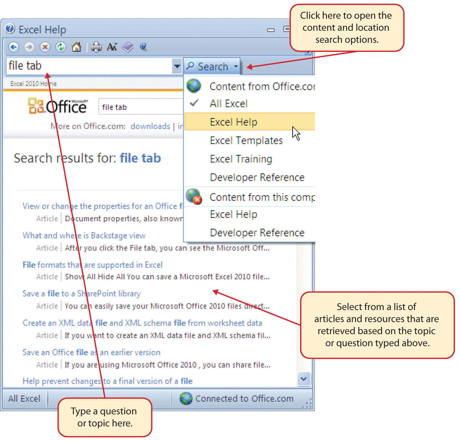
The Help feature provides extensive information about the Excel application. Although some of this information may be stored on your computer, the Help window will automatically connect to the Internet, if you have a live connection, to provide you with resources that can answer most of your questions. You can open the Excel Help window by clicking the question mark in the upper right corner of the screen (see Figure 1.3 "Blank Workbook"). Here you can search for specific topics or type a question in the upper-left side of the window, as shown in Figure 1.16 "Excel Help Window".
Figure 1.16 Excel Help Window
Mouseless Command
Excel Help
- Press the F1 key on your keyboard.
Key Takeaways
- Excel is a powerful tool for processing data for the purposes of making decisions.
- You can find Excel commands throughout the tabs in the Ribbon.
- You can customize the Quick Access Toolbar by adding commands you frequently use.
- You must save your workbook in the Excel 97-2003 file format when sharing workbooks with people who are running Microsoft Office 2003 and older versions.
- Office 2007 can open files created in Office 2010.
- You can add or remove the information that is displayed on the Status Bar.
- The Help window provides you with extensive information about Excel.
Exercises
-
Which of the following responses best defines the notation A1:B15?
- The contents in cell A1 are identical to the contents in cell B15.
- The cells between A1 and B15 are hidden.
- A cell range or contiguous group of cells that begins with cell A1 and include all cells up to and including cell B15.
- A cell link that connects cell A1 to B15.
-
The Spell Check feature is in which tab of the Excel Ribbon?
- Home
- Review
- Data
- Formulas
-
Holding down the CTRL key and pressing the F1 key on your keyboard is used to
- minimize the Ribbon
- open the Excel Help window
- save a workbook
- switch between open workbooks
-
If you are sending an Excel workbook created in Office 2010 to a person who is running Office 2007, you should do the following:
- Use the Save As command to save the workbook in the Office 2007 file format.
- Use the Save As command to save the workbook in the Excel 97-2003 file format.
- Use the Save As command to save the workbook in the Universal Compatibility format.
- Nothing. Office 2007 can open files created in Office 2010.
1.2 Entering, Editing, and Managing Data
Learning Objectives
- Understand how to enter data into a worksheet.
- Examine how to edit data in a worksheet.
- Examine how Auto Fill is used when entering data.
- Understand how to delete data from a worksheet and use the Undo command.
- Examine how to adjust column widths and row heights in a worksheet.
- Understand how to hide columns and rows in a worksheet.
- Examine how to insert columns and rows into a worksheet.
- Understand how to delete columns and rows from a worksheet.
- Learn how to move data to different locations in a worksheet.
In this section, we will begin the development of the workbook shown in Figure 1.1 "Example of an Excel Worksheet with Embedded Chart". The skills covered in this section are typically used in the early stages of developing one or more worksheets in a workbook.
Entering Data
Follow-along file: Excel Objective 1.0 (This is a blank workbook that was named in the previous section. If you skipped the previous section, open a new workbook and save it with the file name “Excel Objective 1.0.”)
We will begin building the workbook shown in Figure 1.1 "Example of an Excel Worksheet with Embedded Chart" by manually entering data into the worksheet. There are other ways in which you can bring data into an Excel worksheet, such as importing data from a website or a Microsoft Access database. However, we will demonstrate these other methods later. The following steps explain how the column headings in Row 2 are typed into the worksheet:
- Activate cell location A2 on the worksheet.
- Type the word Month.
- Press the RIGHT ARROW key. This will enter the word into cell A2 and activate the next cell to the right.
- Type Unit Sales and press the RIGHT ARROW key.
-
Repeat step 4 for the words Average Price and Sales Dollars.
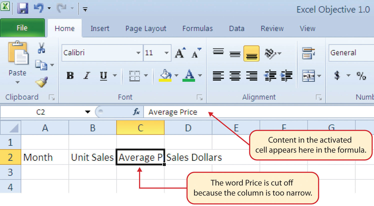
Figure 1.17 "Entering Column Headings into a Worksheet" shows how your worksheet should appear after you have typed the column headings into Row 2. Notice that the word Price in cell location C2 is not visible. This is because the column is too narrow to fit the entry you typed. We will examine formatting techniques to correct this problem in the next section.
Figure 1.17 Entering Column Headings into a Worksheet
Integrity Check
Column Headings
It is critical to include column headings that accurately describe the data in each column of a worksheet. In professional environments, you will likely be sharing Excel workbooks with coworkers. Good column headings reduce the chance of someone misinterpreting the data contained in a worksheet, which could lead to costly errors depending on your career.
- Activate cell location B3.
- Type the number 2670 and press the ENTER key. After you press the ENTER key, cell B4 will be activated. Using the ENTER key is an efficient way to enter data vertically down a column.
-
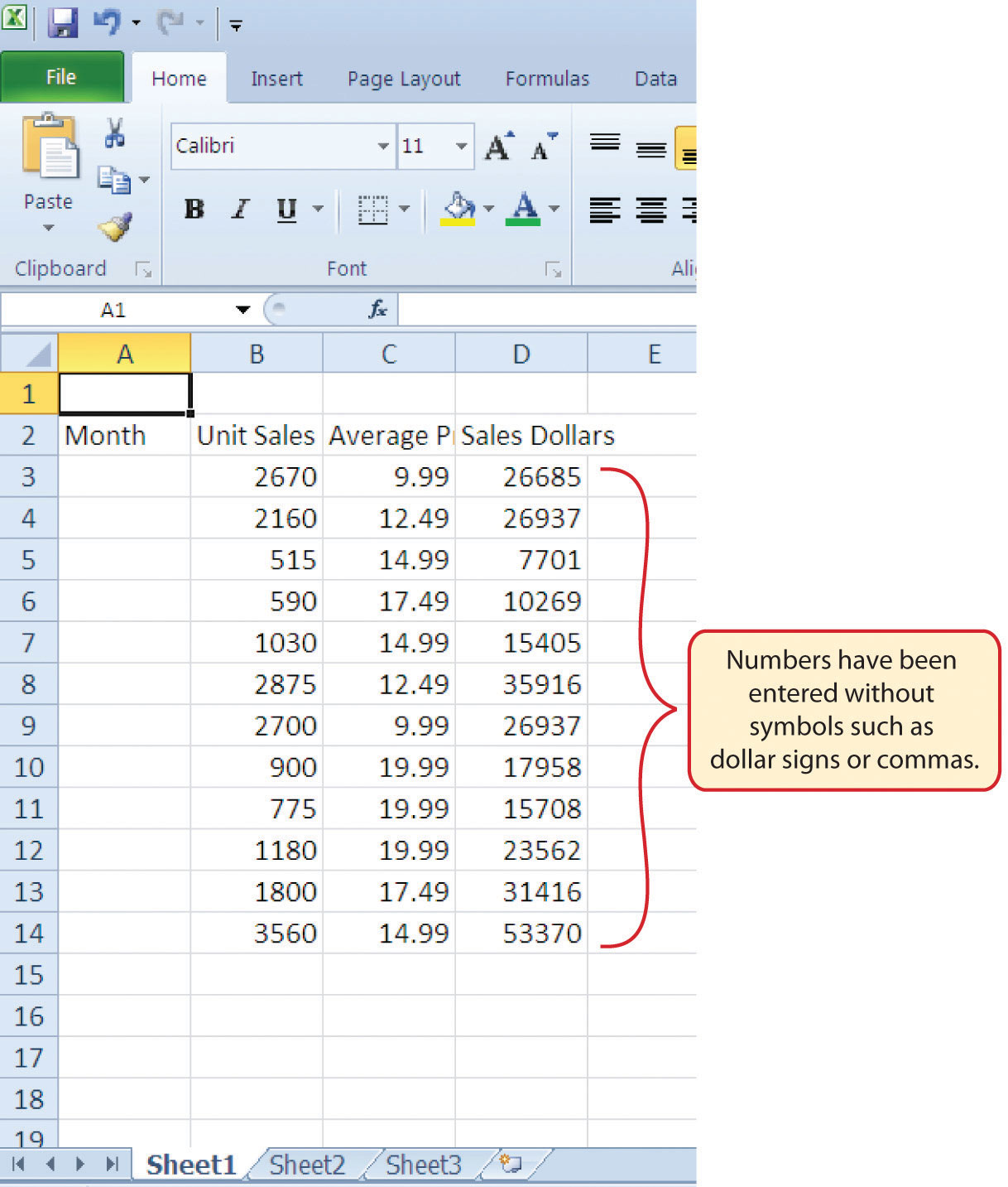
Repeat step 7 by entering the following numbers in cells B4 through B14: 2160, 515, 590, 1030, 2875, 2700, 900, 775, 1180, 1800, and 3560.
Why?
Avoid Formatting Symbols When Entering Numbers
When typing numbers into an Excel worksheet, it is best to avoid adding any formatting symbols such as dollar signs and commas. Although Excel allows you to add these symbols while typing numbers, it slows down the process of entering data. It is more efficient to use Excel’s formatting features to add these symbols to numbers after you type them into a worksheet.
- Activate cell location C3.
- Type the number 9.99 and press the ENTER key.
- Repeat step 10 by entering the following numbers in cells C4 through C14: 12.49, 14.99, 17.49, 14.99, 12.49, 9.99, 19.99, 19.99, 19.99, 17.49, and 14.99.
- Activate cell location D3.
- Type the number 26685 and press the ENTER key.
- Repeat step 13 by entering the following numbers in cells D4 through D14: 26937, 7701, 10269, 15405, 35916, 26937, 17958, 15708, 23562, 31416, and 53370.
Integrity Check
Data Entry
It is very important to proofread your worksheet carefully, especially when you have entered numbers. Transposing numbers when entering data manually into a worksheet is a common error. For example, the number 563 could be transposed to 536. Such errors can seriously compromise the integrity of your workbook.
Figure 1.18 "Completed Data Entry for Columns B, C, and D" shows how your worksheet should appear after entering the data. Check your numbers carefully to make sure they are accurately entered into the worksheet.
Figure 1.18 Completed Data Entry for Columns B, C, and D
Editing Data
Follow-along file: Excel Objective 1.0 (Use file Excel Objective 1.01 if you are starting with this skill.)
Data that has been entered in a cell can be changed by double clicking the cell location or using the Formula BarThe area just above the column letters on a worksheet. It can be used for entering data into cells as well as for editing data that already exists in cells.. You may have noticed that as you were typing data into a cell location, the data you typed appeared in the Formula Bar. The Formula Bar can be used for entering data into cells as well as for editing data that already exists in a cell. The following steps provide an example of entering and then editing data that has been entered into a cell location:
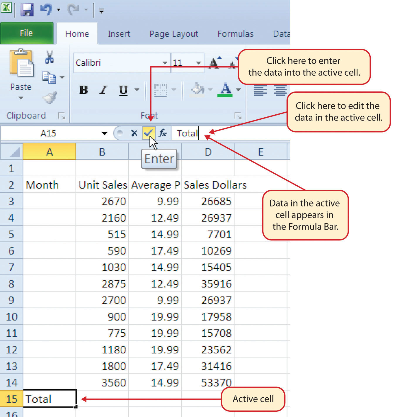
- Activate cell A15 in the Sheet1 worksheet.
- Type the abbreviation Tot and press the ENTER key.
- Click cell A15.
- Move the mouse pointer up to the Formula Bar. You will see the pointer turn into a cursor. Move the cursor to the end of the abbreviation Tot and left click.
- Type the letters al to complete the word Total.
-
Click the checkmark to the left of the Formula Bar (see Figure 1.19 "Using the Formula Bar to Edit and Enter Data"). This will enter the change into the cell.
Figure 1.19 Using the Formula Bar to Edit and Enter Data
- Double click cell A15.
- Add a space after the word Total and type the word Sales.
- Press the ENTER key.
Mouseless Command
Editing Data in a Cell
- Activate the cell that is to be edited and press the F2 key on your keyboard.
Auto Fill
Follow-along file: Excel Objective 1.0 (Use file Excel Objective 1.02 if you are starting with this skill.)
The Auto FillAn Excel feature used to complete data in either a quantitative or qualitative sequence. It can also be used to copy and paste data in a worksheet. feature is a valuable tool when manually entering data into a worksheet. This feature has many uses, but it is most beneficial when you are entering data in a defined sequence, such as the numbers 2, 4, 6, 8, and so on, or nonnumeric data such as the days of the week or months of the year. The following steps demonstrate how Auto Fill can be used to enter the months of the year in Column A:
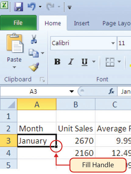
- Activate cell A3 in the Sheet1 worksheet.
- Type the word January and press the ENTER key.
- Activate cell A3 again.
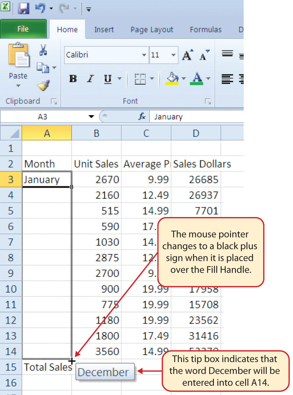
-
Move the mouse pointer to the lower right corner of cell A3. You will see a small square in this corner of the cell; this is called the Fill HandleA small square in lower right corner of an activated cell. When the mouse pointer gets close to the Fill Handle, the white block plus sign turns into a black plus sign. (see Figure 1.20 "Fill Handle"). When the mouse pointer gets close to the Fill Handle, the white block plus sign will turn into a black plus sign.
Figure 1.20 Fill Handle
-
Left click and drag the Fill Handle to cell A14. Notice that the Auto Fill tip box indicates what month will be placed into each cell (see Figure 1.21 "Using Auto Fill to Enter the Months of the Year"). Release the left mouse button when the tip box reads “December.”
Figure 1.21 Using Auto Fill to Enter the Months of the Year
Once you release the left mouse button, all twelve months of the year should appear in the cell range A3:A14, as shown in Figure 1.22 "Auto Fill Options Button". You will also see the Auto Fill Options button. By clicking this button, you have several options for inserting data into a group of cells.
Figure 1.22 Auto Fill Options Button
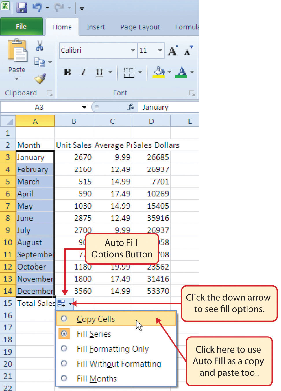
- Left click the Auto Fill Options button.
- Left click the Copy Cells option. This will change the months in the range A4:A14 to January.
- Left click the Auto Fill Options button again.
- Left click the Fill Months option to return the months of the year to the cell range A4:A14. The Fill Series option will provide the same result.
Deleting Data and the Undo Command
Follow-along file: Excel Objective 1.0 (Use file Excel Objective 1.03 if you are starting with this skill.)
There are several methods for removing data from a worksheet, a few of which are demonstrated here. With each method, you use the Undo command. This is a helpful command in the event you mistakenly remove data from your worksheet. The following steps demonstrate how you can delete data from a cell or range of cells:
- Activate cell C2 by placing the mouse pointer over the cell and clicking the left mouse button.
- Press the DELETE key on your keyboard. This removes the contents of the cell.
- Highlight the range C3:C14 by placing the mouse pointer over cell C3. Then left click and drag the mouse pointer down to cell C14.
- Place the mouse pointer over the Fill Handle. You will see the white block plus sign change to a black plus sign.
-
Left click and drag the mouse pointer up to cell C3 (see Figure 1.23 "Using Auto Fill to Delete Contents of Cell"). Release the mouse button. The contents in the range C3:C14 will be removed.
Figure 1.23 Using Auto Fill to Delete Contents of Cell
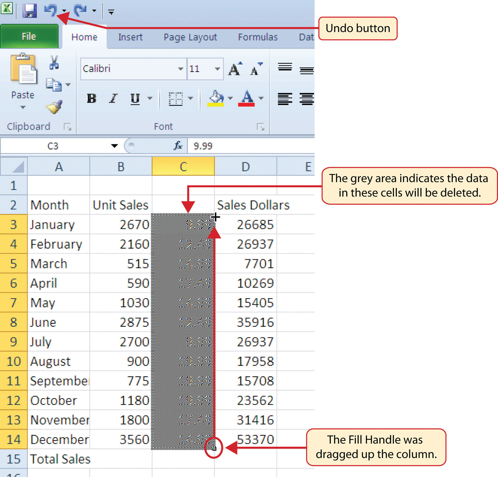
- Click the Undo button in the Quick Access Toolbar (see Figure 1.3 "Blank Workbook"). This should replace the data in the range C3:C14.
-
Click the Undo button again. This should replace the data in cell C2.
Mouseless Command
Undo Command
- Hold down the CTRL key while pressing the letter Z on your keyboard.
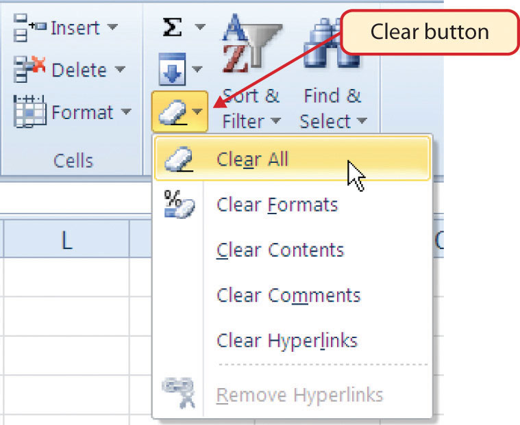
- Highlight the range C2:C14 by placing the mouse pointer over cell C2. Then left click and drag the mouse pointer down to cell C14.
- Click the Clear button in the Home tab of the Ribbon, which is next to the Cells group of commands (see Figure 1.24 "Clear Command Drop-Down Menu"). This opens a drop-down menu that contains several options for removing or clearing data from a cell. Notice that you also have options for clearing just the formats in a cell or the hyperlinks in a cell.
- Click the Clear All option. This removes the data in the cell range.
- Click the Undo button. This replaces the data in the range C2:C14.
Figure 1.24 Clear Command Drop-Down Menu
Adjusting Columns and Rows
Follow-along file: Excel Objective 1.0 (Use file Excel Objective 1.03 if you are starting with this skill.)
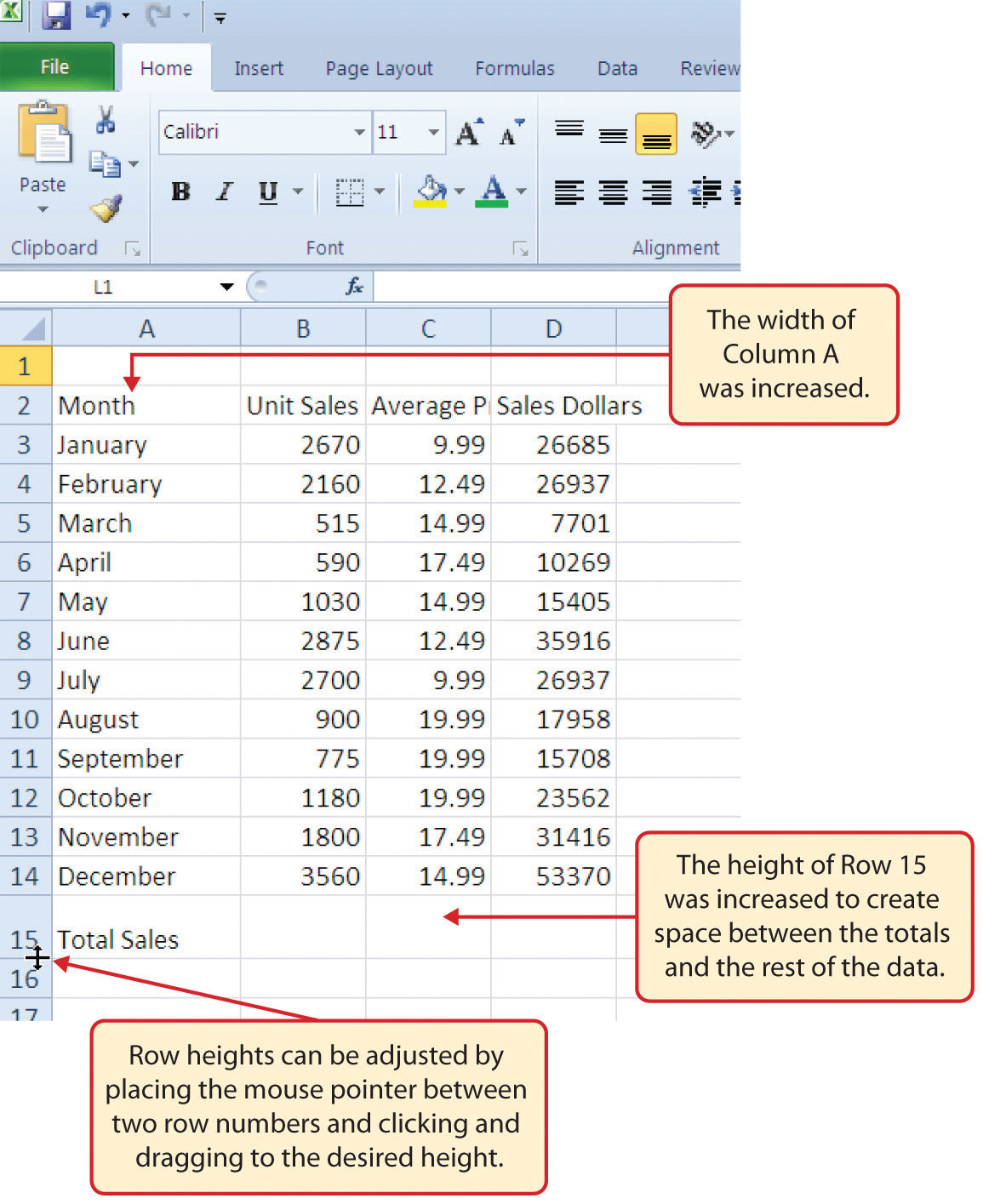
In Figure 1.22 "Auto Fill Options Button", there are a few entries that appear cut off. For example, the last letter of the word September cannot be seen in cell A11. This is because the column is too narrow for this word. The columns and rows on an Excel worksheet can be adjusted to accommodate the data that is being entered into a cell. The following steps explain how to adjust the column widths and row heights in a worksheet:
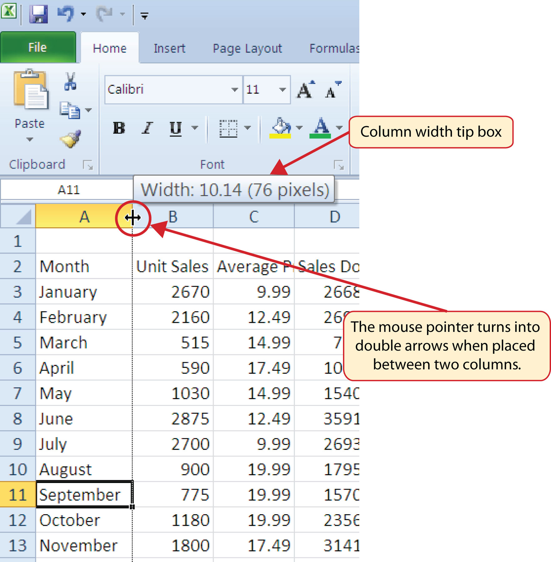
- Bring the mouse pointer between Column A and Column B in the Sheet1 worksheet, as shown in Figure 1.25 "Adjusting Column Widths". You will see the white block plus sign turn into double arrows.
- Left click and drag the column to the right so the entire word September in cell A11 can be seen. As you drag the column, you will see the column width tip boxA box that appears when the width of a column is being adjusted using the click-and-drag method. It displays the number of characters that will fit into the column using Calibri 11-point font.. This box displays the number of characters that will fit into the column using the Calibri 11-point font.
-
Release the left mouse button.
Figure 1.25 Adjusting Column Widths
You may find that using the click-and-drag method is inefficient if you need to set a specific character width for one or more columns. Steps 4 through 7 illustrate a second method for adjusting column widths when using a specific number of characters:
- Activate any cell location in Column A by moving the mouse pointer over a cell location and clicking the left mouse button. You can highlight cell locations in multiple columns if you are setting the same character width for more than one column.
- In the Home tab of the Ribbon, left click the Format button in the Cells group (see Figure 1.26 "Cells Group in the Home Tab").
- Click the Column Width option from the drop-down menu (see Figure 1.27 "Format Drop-Down Menu"). This will open the Column Width dialog box.
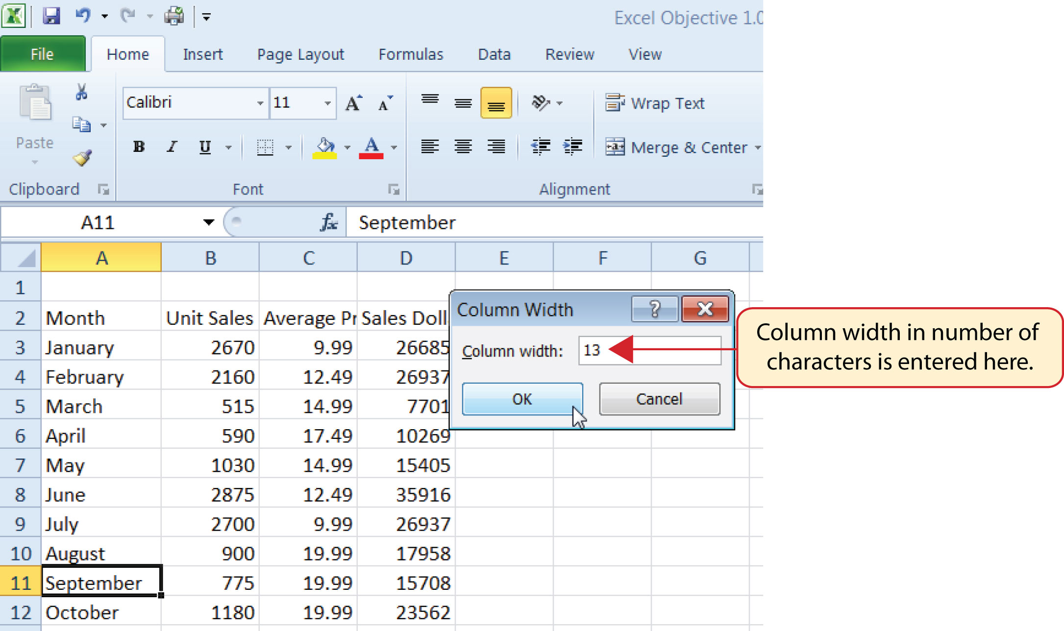
-
Type the number 13 and click the OK button on the Column Width dialog box. This will set Column A to this character width (see Figure 1.28 "Column Width Dialog Box").
Figure 1.26 Cells Group in the Home Tab
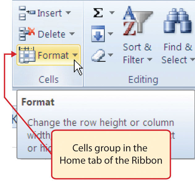
Figure 1.27 Format Drop-Down Menu
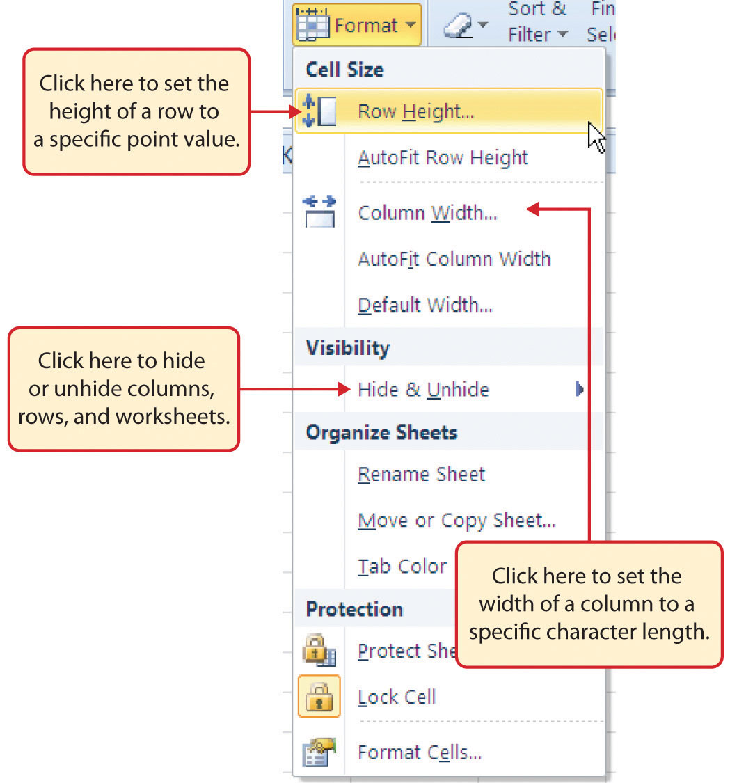
Figure 1.28 Column Width Dialog Box
Mouseless Command
Column Width
- Press the ALT key on your keyboard, then press the letters H, O, and W one at a time.
Steps 8 through 10 demonstrate how to adjust row height, which is similar to adjusting column width:
- Activate cell A15 by placing the mouse pointer over the cell and clicking the left mouse button.
- In the Home tab of the Ribbon, left click the Format button in the Cells group (see Figure 1.26 "Cells Group in the Home Tab").
- Click the Row Height option from the drop-down menu (see Figure 1.27 "Format Drop-Down Menu"). This will open the Row Height dialog box.
- Type the number 24 and click the OK button on the Row Height dialog box. This will set Row 15 to a height of 24 points. A pointMetric used when measuring the height of a row; equivalent to approximately 1/72 of an inch. is equivalent to approximately 1/72 of an inch. This adjustment in row height was made to create space between the totals for this worksheet and the rest of the data.
Mouseless Command
Row Height
- Press the ALT key on your keyboard, then press the letters H, O, and H one at a time.
Figure 1.29 "Excel Objective 1.0 with Column A and Row 15 Adjusted" shows the appearance of the worksheet after Column A and Row 15 are adjusted.
Figure 1.29 Excel Objective 1.0 with Column A and Row 15 Adjusted
Skill Refresher: Adjusting Columns and Rows
- Activate at least one cell in the row or column you are adjusting.
- Click the Home tab of the Ribbon.
- Click the Format button in the Cells group.
- Click either Row Height or Column Width from the drop-down menu.
- Enter the Row Height in points or Column Width in characters in the dialog box.
- Click the OK button.
Hiding Columns and Rows
Follow-along file: Excel Objective 1.0 (Use file Excel Objective 1.04 if you are starting with this skill.)
In addition to adjusting the columns and rows on a worksheet, you can also hide columns and rows. This is a useful technique for enhancing the visual appearance of a worksheet that contains data that is not necessary to display. These features will be demonstrated using the Excel Objective 1.0 workbook. However, there is no need to have hidden columns or rows for this worksheet. The use of these skills here will be for demonstration purposes only.
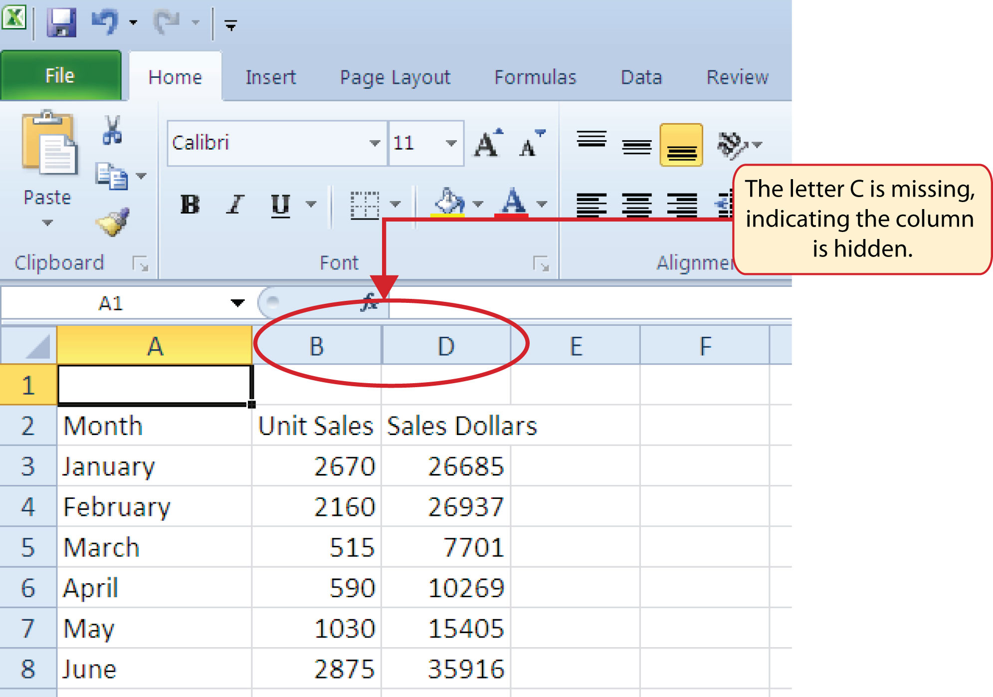
- Activate cell C1 in the Sheet1 worksheet by placing the mouse pointer over the cell location and clicking the left mouse button.
- Click the Format button in the Home tab of the Ribbon.
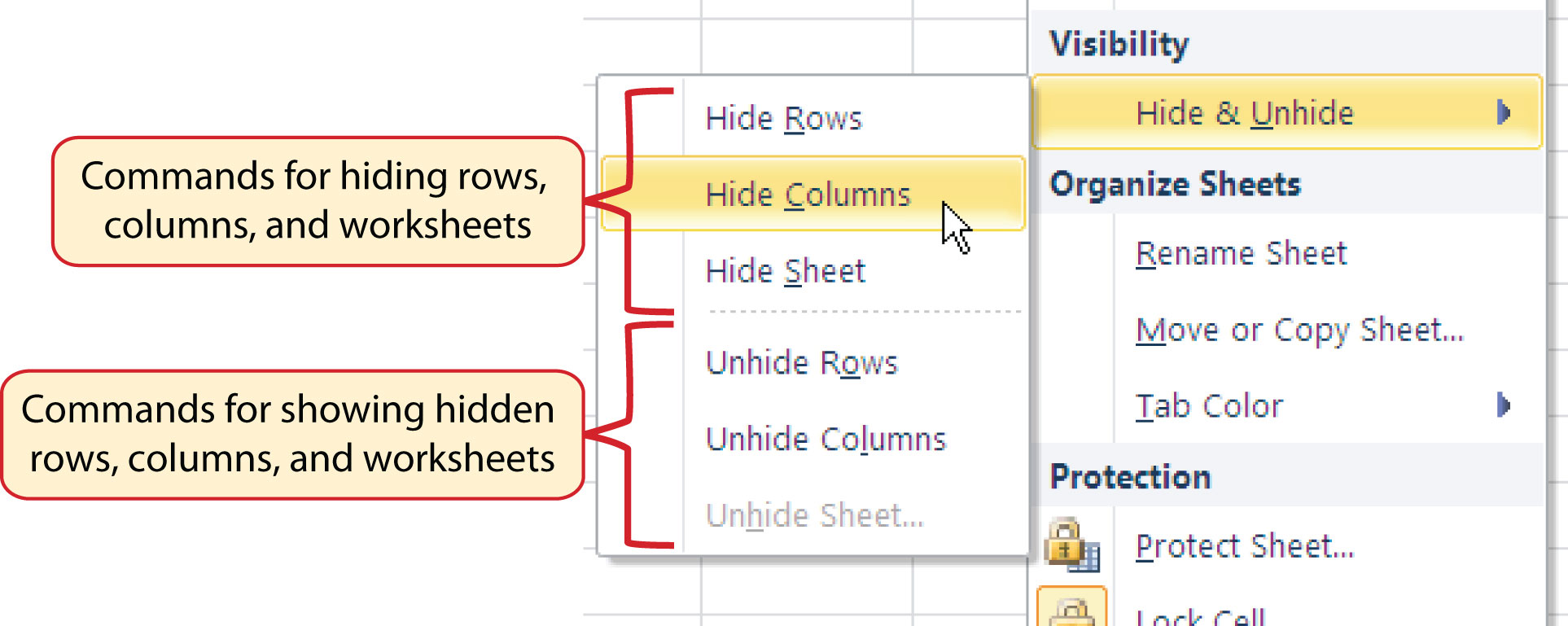
- Place the mouse pointer over the Hide & Unhide option in the drop-down menu (see Figure 1.27 "Format Drop-Down Menu"). This will open a submenu of options.
-
Click the Hide Columns option in the submenu of options (see Figure 1.30 "Hide & Unhide Submenu"). This will hide Column C.
Figure 1.30 Hide & Unhide Submenu
Mouseless Command
Hiding Columns
- Hold down the CTRL key while pressing the number 0 on your keyboard.
Figure 1.31 "Hidden Column" shows the workbook with Column C hidden in the Sheet1 worksheet. You can tell a column is hidden by the missing letter C.
Figure 1.31 Hidden Column
To unhide a column, follow these steps:
- Highlight the range B1:D1 by activating cell B1 and clicking and dragging over to cell D1.
- Click the Format button in the Home tab of the Ribbon.
- Place the mouse pointer over the Hide & Unhide option in the drop-down menu (see Figure 1.27 "Format Drop-Down Menu").
-
Click the Unhide Columns option in the submenu of options (see Figure 1.30 "Hide & Unhide Submenu"). Column C will now be visible on the worksheet.
Mouseless Command
Unhiding Columns
- Highlight cells on either side of the hidden column(s), then hold down the CTRL key and the SHIFT key while pressing the close parenthesis key ()) on your keyboard.
The following steps demonstrate how to hide rows, which is similar to hiding columns:
- Activate cell A3 in the Sheet1 worksheet by placing the mouse pointer over the cell location and clicking the left mouse button.
- Click the Format button in the Home tab of the Ribbon.
- Place the mouse pointer over the Hide & Unhide option in the drop-down menu (see Figure 1.27 "Format Drop-Down Menu"). This will open a submenu of options.
-
Click the Hide Rows option in the submenu of options (see Figure 1.30 "Hide & Unhide Submenu"). This will hide Row 3.
Mouseless Command
Hiding Rows
- Hold down the CTRL key while pressing the number 9 key on your keyboard.
To unhide a row, follow these steps:
- Highlight the range A2:A4 by activating cell A2 and clicking and dragging over to cell A4.
- Click the Format button in the Home tab of the Ribbon.
- Place the mouse pointer over the Hide & Unhide option in the drop-down menu (see Figure 1.27 "Format Drop-Down Menu").
- Click the Unhide Rows option in the submenu of options (see Figure 1.30 "Hide & Unhide Submenu"). Row 3 will now be visible on the worksheet.
Mouseless Command
Unhiding Rows
- Highlight cells above and below the hidden row(s), then hold down the CTRL key and the SHIFT key while pressing the open parenthesis key (() on your keyboard.
Integrity Check
Hidden Rows and Columns
In most careers, it is common for professionals to use Excel workbooks that have been designed by a coworker. Before you use a workbook developed by someone else, always check for hidden rows and columns. You can quickly see whether a row or column is hidden if a row number or column letter is missing.
Skill Refresher: Hiding Columns and Rows
- Activate at least one cell in the row(s) or column(s) you are hiding.
- Click the Home tab of the Ribbon.
- Click the Format button in the Cells group.
- Place the mouse pointer over the Hide & Unhide option.
- Click either the Hide Rows or Hide Columns option.
Skill Refresher: Unhiding Columns and Rows
- Highlight the cells above and below the hidden row(s) or to the left and right of the hidden column(s).
- Click the Home tab of the Ribbon.
- Click the Format button in the Cells group.
- Place the mouse pointer over the Hide & Unhide option.
- Click either the Unhide Rows or Unhide Columns option.
Inserting Columns and Rows
Follow-along file: Excel Objective 1.0 (Use file Excel Objective 1.04 if you are starting with this skill.)
Using Excel workbooks that have been created by others is a very efficient way to work because it eliminates the need to create data worksheets from scratch. However, you may find that to accomplish your goals, you need to add additional columns or rows of data. In this case, you can insert blank columns or rows into a worksheet. The following steps demonstrate how to do this:
- Activate cell C1 in the Sheet1 worksheet by placing the mouse pointer over the cell location and clicking the left mouse button.
-
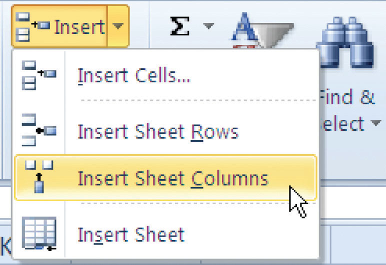
Click the down arrow on the Insert button in the Home tab of the Ribbon (see Figure 1.32 "Insert Button (Down Arrow)").
Figure 1.32 Insert Button (Down Arrow)
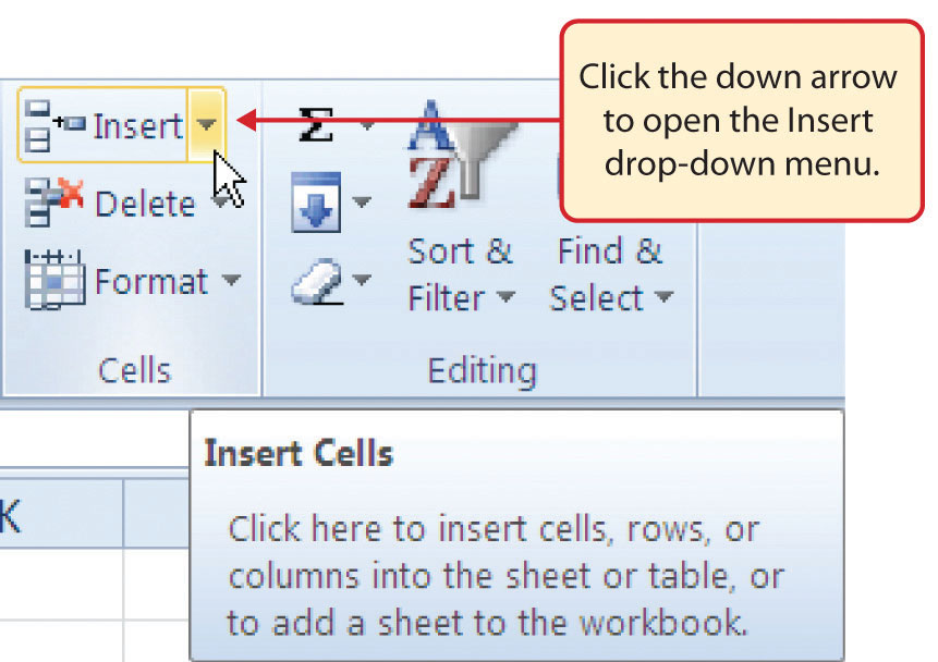
-
Click the Insert Sheet Columns option from the drop-down menu (see Figure 1.33 "Insert Drop-Down Menu"). A blank column will be inserted to the left of Column C. The contents that were previously in Column C now appear in Column D. Note that columns are always inserted to the left of the activated cell.
Mouseless Command
Inserting Columns
- Press the ALT key and then the letters H, I, and C one at a time. A column will be inserted to the left of the activated cell.
Figure 1.33 Insert Drop-Down Menu
- Activate cell A3 in the Sheet1 worksheet by placing the mouse pointer over the cell location and clicking the left mouse button.
- Click the down arrow on the Insert button in the Home tab of the Ribbon (see Figure 1.32 "Insert Button (Down Arrow)").
- Click the Insert Sheet Rows option from the drop-down menu (see Figure 1.33 "Insert Drop-Down Menu"). A blank row will be inserted above Row 3. The contents that were previously in Row 3 now appear in Row 4. Note that rows are always inserted above the activated cell.
Mouseless Command
Inserting Rows
- Press the ALT key and then the letters H, I, and R one at a time. A row will be inserted above the activated cell.
Skill Refresher: Inserting Columns and Rows
- Activate the cell to the right of the desired blank column or below the desired blank row.
- Click the Home tab of the Ribbon.
- Click the down arrow on the Insert button in the Cells group.
- Click either the Insert Sheet Columns or Insert Sheet Rows option.
Moving Data
Follow-along file: Excel Objective 1.0 (Use file Excel Objective 1.05 if you skipped the previous skill and are starting with this skill.)
Once data are entered into a worksheet, you have the ability to move it to different locations. The following steps demonstrate how to move data to different locations on a worksheet:
- Highlight the range D2:D15 by activating cell D2 and clicking and dragging down to cell D15.
-
Bring the mouse pointer to the left edge of cell D2. You will see the white block plus sign change to cross arrows (see Figure 1.34 "Moving Data"). This indicates that you can left click and drag the data to a new location.
Figure 1.34 Moving Data
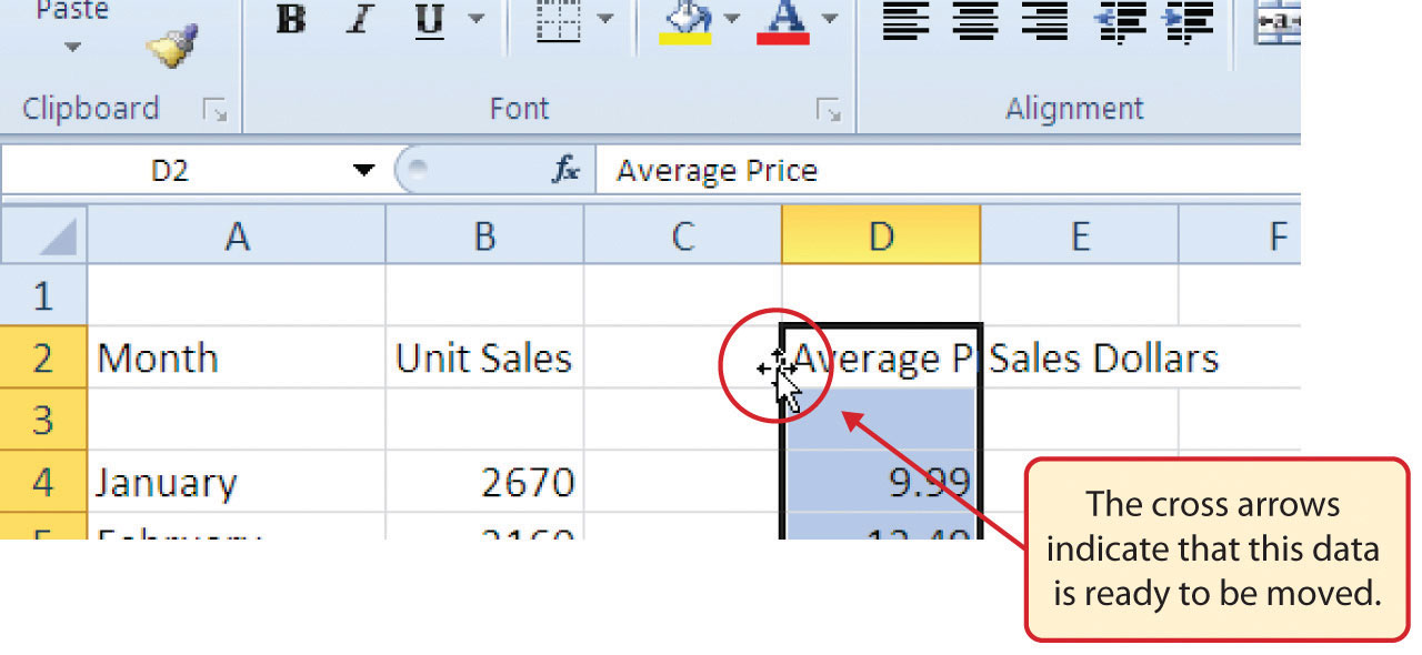
- Left click and drag the mouse pointer to cell C2.
- Release the left mouse button. The data now appears in Column C.
- Click the Undo button in the Quick Access Toolbar. This moves the data back to Column D.
Integrity Check
Moving Data
Before moving data on a worksheet, make sure you identify all the components that belong with the series you are moving. For example, if you are moving a column of data, make sure the column heading is included. Also, make sure all values are highlighted in the column before moving it.
Deleting Columns and Rows
Follow-along file: Excel Objective 1.0 (Use file Excel Objective 1.05 if you are starting with this skill.)
You may need to delete entire columns or rows of data from a worksheet. This need may arise if you need to remove either blank columns or rows from a worksheet or columns and rows that contain data. The methods for removing cell contents were covered earlier and can be used to delete unwanted data. However, if you do not want a blank row or column in your workbook, you can delete it using the following steps:
- Activate cell A3 by placing the mouse pointer over the cell location and clicking the left mouse button.
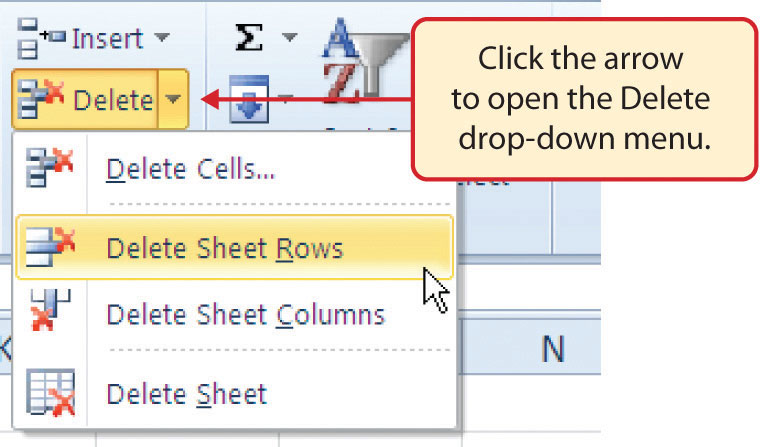
- Click the down arrow on the Delete button in the Cells group in the Home tab of the Ribbon.
-
Click the Delete Sheet Rows option from the drop-down menu (see Figure 1.35 "Delete Drop-Down Menu"). This removes Row 3 and shifts all the data (below Row 2) in the worksheet up one row.
Mouseless Command
Deleting Rows
- Press the ALT key and then the letters H, D, and R one at a time. The row with the activated cell will be deleted.
Figure 1.35 Delete Drop-Down Menu
- Activate cell C1 by placing the mouse pointer over the cell location and clicking the left mouse button.
- Click the down arrow on the Delete button in the Cells group in the Home tab of the Ribbon.
- Click the Delete Sheet Columns option from the drop-down menu (see Figure 1.35 "Delete Drop-Down Menu"). This removes Column C and shifts all the data in the worksheet (to the right of Column B) over one column to the left.
Mouseless Command
Deleting Columns
- Press the ALT key and then the letters H, D, and C one at a time. The column with the activated cell will be deleted.
Skill Refresher: Deleting Columns and Rows
- Activate any cell in the row or column that is to be deleted.
- Click the Home tab of the Ribbon.
- Click the down arrow on the Delete button in the Cells group.
- Click either the Delete Sheet Columns or the Delete Sheet Rows option.
Key Takeaways
- Column headings should be used in a worksheet and should accurately describe the data contained in each column.
- Using symbols such as dollar signs when entering numbers into a worksheet can slow down the data entry process.
- Worksheets must be carefully proofread when data has been manually entered.
- The Undo command is a valuable tool for recovering data that was deleted from a worksheet.
- When using a worksheet that was developed by someone else, look carefully for hidden column or rows.
Exercises
-
When entering numeric data into an Excel worksheet, you should omit symbols such as commas or dollar signs because:
- These numbers will not be usable in mathematical functions or formulas.
- Excel will convert this to text data.
- Excel will not accept these entries into a cell location.
- It slows down the data entry process.
-
Which of the following statements is true with respect to editing the content in a cell location?
- Activate the cell location and press the F2 key on your keyboard to edit the data in the cell.
- Double click the cell location to edit the data in a cell location.
- Activate the cell location, click the Formula Bar, and make any edits for the cell location in the Formula Bar.
- All of the above are true.
-
Which of the following will enable you to identify hidden columns in a worksheet?
- The column letter appears in a tip box when the mouse pointer is moved over a hidden column.
- Clicking the Page Layout View button in the View tab of the Ribbon shows all columns in the worksheet and shades hidden columns.
- The column letters that appear above the columns in a worksheet will be missing for hidden columns.
- Click the Hidden Columns indicator in the Status Bar.
-
Which of the following is true with respect to inserting blank rows into a worksheet?
- Blank rows are inserted above the activated cell or cell range in a worksheet.
- Blank rows are always inserted in the center of a cell range. At least two or more cells in a worksheet must be highlighted before a row can be inserted.
- The command for inserting blank rows and columns can be found by clicking the Format button in the Home tab of the Ribbon.
- When inserting blank rows into a worksheet, the Undo button is disabled. You must use the Delete button in the Home tab of the Ribbon to remove unwanted blank rows.
1.3 Formatting and Data Analysis
Learning Objectives
- Use formatting techniques to enhance the appearance of a worksheet.
- Understand how to align data in cell locations.
- Examine how to enter multiple lines of text in a cell location.
- Understand how to add borders to a worksheet.
- Examine how to use the AutoSum feature to calculate totals.
- Understand how to insert a chart into a worksheet.
- Use the Cut, Copy, and Paste commands to manipulate the data on a worksheet.
- Examine how to use the Sort command to rank data on a worksheet.
- Understand how to move, rename, insert, and delete worksheet tabs.
This section addresses formatting commands that can be used to enhance the visual appearance of a worksheet. It also provides an introduction to mathematical calculations and charts. The skills introduced in this section will give you powerful tools for analyzing the data that we have been working with in this workbook and will highlight how Excel is used to make key decisions in virtually any career.
Formatting Data and Cells
Follow-along file: Excel Objective 1.0 (Use file Excel Objective 1.04 if you are starting with this skill.)
Enhancing the visual appearance of a worksheet is a critical step in creating a valuable tool for you or your coworkers when making key decisions. The following steps demonstrate several fundamental formatting skills that will be applied to the workbook that we are developing for this chapter. Several of these formatting skills are identical to ones that you may have already used in other Microsoft applications such as Microsoft® Word® or Microsoft® PowerPoint®.
- Highlight the range A2:D2 in the Sheet1 worksheet by placing the mouse pointer over cell A2 and left clicking and dragging to cell D2.
-
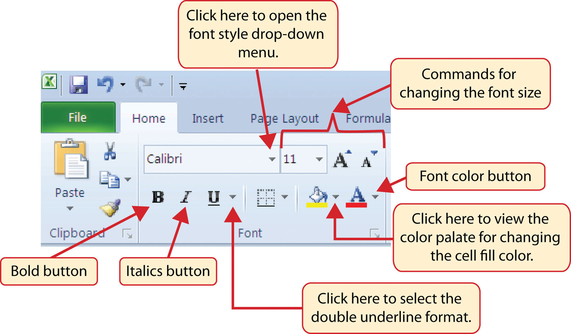
Click the Bold button in the Font group of commands in the Home tab of the Ribbon (see Figure 1.36 "Font Group of Commands").
Figure 1.36 Font Group of Commands
Mouseless Command
Bold Format
- Hold the CTRL key while pressing the letter B on your keyboard.
- Highlight the range A15:D15 by placing the mouse pointer over cell A15 and left clicking and dragging to cell D15.
- Click the Bold button in the Font group of commands in the Home tab of the Ribbon.
- Click the Italics button in the Font group of commands in the Home tab of the Ribbon (see Figure 1.36 "Font Group of Commands").
-
Click the Underline button in the Font group of commands in the Home tab of the Ribbon (see Figure 1.36 "Font Group of Commands"). Notice that there is a drop-down arrow next to the Underline button. This is for selecting a double underline format, which is common in careers that deal with accounting or budgeting activities.
Mouseless Command
Italics Format
- Hold the CTRL key while pressing the letter I on your keyboard.
Mouseless Command
Underline Format
- Hold the CTRL key while pressing the letter U on your keyboard.
Why?
Format Column Headings and Totals
Applying formatting enhancements to the column headings and column totals in a worksheet is a very important technique, especially if you are sharing a workbook with other people. These formatting techniques allow users of the worksheet to clearly see the column headings that define the data. In addition, the column totals usually contain the most important data on a worksheet with respect to making decisions, and formatting techniques allow users to quickly see this information.
- Highlight the range B3:B14 by placing the mouse pointer over cell B3 and left clicking and dragging down to cell B14.
-
Click the Comma Style button in the Number group of commands in the Home tab of the Ribbon (see Figure 1.37 "Number Group of Commands").
Figure 1.37 Number Group of Commands

- Click the Decrease Decimal button in the Number group of commands in the Home tab of the Ribbon (see Figure 1.37 "Number Group of Commands").
- The numbers will also be reduced to zero decimal places.
- Highlight the range C3:C14 by placing the mouse pointer over cell C3 and left clicking and dragging down to cell C14.
- Click the Accounting Number Format button in the Number group of commands in the Home tab of the Ribbon (see Figure 1.37 "Number Group of Commands"). This will add the US currency symbol and two decimal places to the values. This format is common when working with pricing data.
- Highlight the range D3:D14 by placing the mouse pointer over cell D3 and left clicking and dragging down to cell D14.
- Again, this will add the US currency symbol to the values as well as two decimal places.
- Click the Decrease Decimal button in the Number group of commands in the Home tab of the Ribbon.
- This will add the US currency symbol to the values and reduce the decimal places to zero.
- Highlight the range A1:D1 by placing the mouse pointer over cell A1 and left clicking and dragging over to cell D1.
-
Click the down arrow next to the Fill Color button in the Font group of commands in the Home tab of the Ribbon (see Figure 1.38 "Fill Color Palette").
Figure 1.38 Fill Color Palette
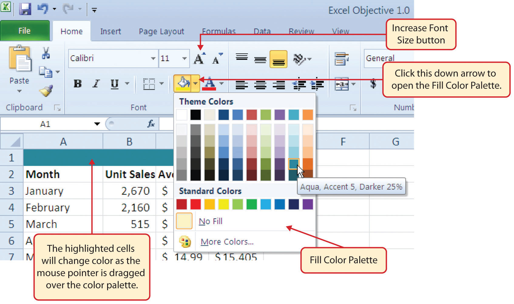
- Click the Aqua, Accent 5, Darker 25% color from the palette (see Figure 1.38 "Fill Color Palette"). Notice that as you move the mouse pointer over the color palette, you will see a preview of how the color will appear in the highlighted cells.
- Click the down arrow next to the Font Color button in the Font group of commands in the Home tab of the Ribbon (see Figure 1.36 "Font Group of Commands").
- This change will be visible once text is typed into the highlighted cells.
- Click the Increase Font Size button in the Font group of commands in the Home tab of the Ribbon (see Figure 1.38 "Fill Color Palette").
- Highlight the range A1:D15 by placing the mouse pointer over cell A1 and left clicking and dragging down to cell D15.
- Click the drop-down arrow on the right side of the Font button in the Home tab of the Ribbon (see Figure 1.36 "Font Group of Commands").
- Notice that as you move the mouse pointer over the font style options, you can see the font change in the highlighted cells.
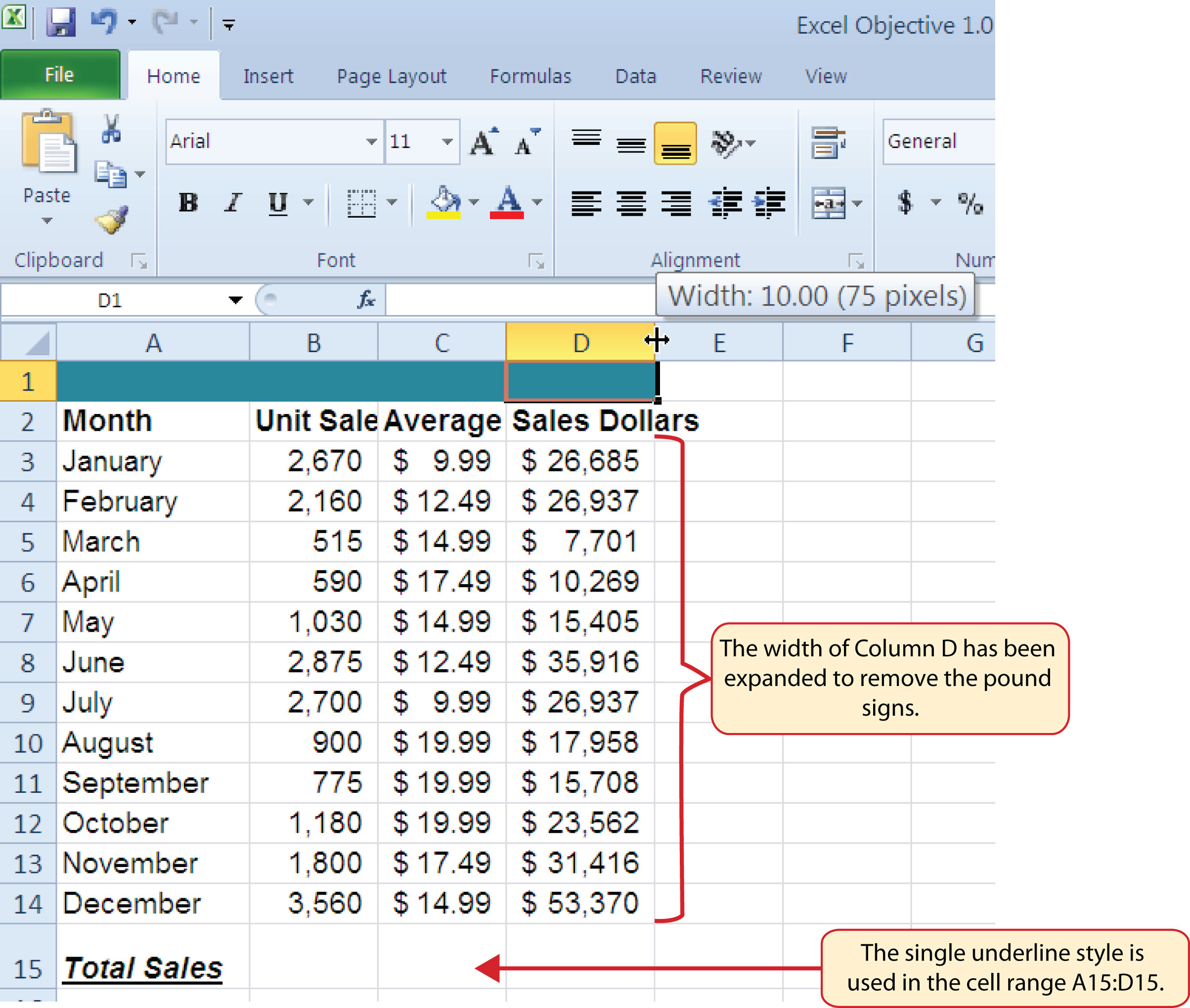
- Expand the row width of Column D to 10 characters.
Why?
Pound Signs (####) Appear in Columns
When a column is too narrow for a long number, Excel will automatically convert the number to a series of pound signs (####). In the case of words or text data, Excel will only show the characters that fit in the column. However, this is not the case with numeric data because it can give the appearance of a number that is much smaller than what is actually in the cell. To remove the pound signs, increase the width of the column.
Figure 1.39 "Formatting Techniques Applied" shows how the Sheet1 worksheet should appear after the formatting techniques are applied.
Figure 1.39 Formatting Techniques Applied
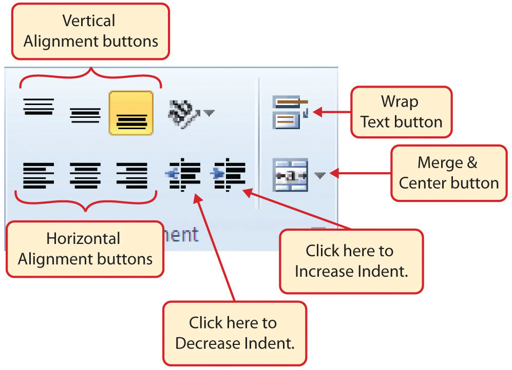
Data Alignment (Wrap Text, Merge Cells, and Center)
Follow-along file: Excel Objective 1.0 (Use file Excel Objective 1.06 if you are starting with this skill.)
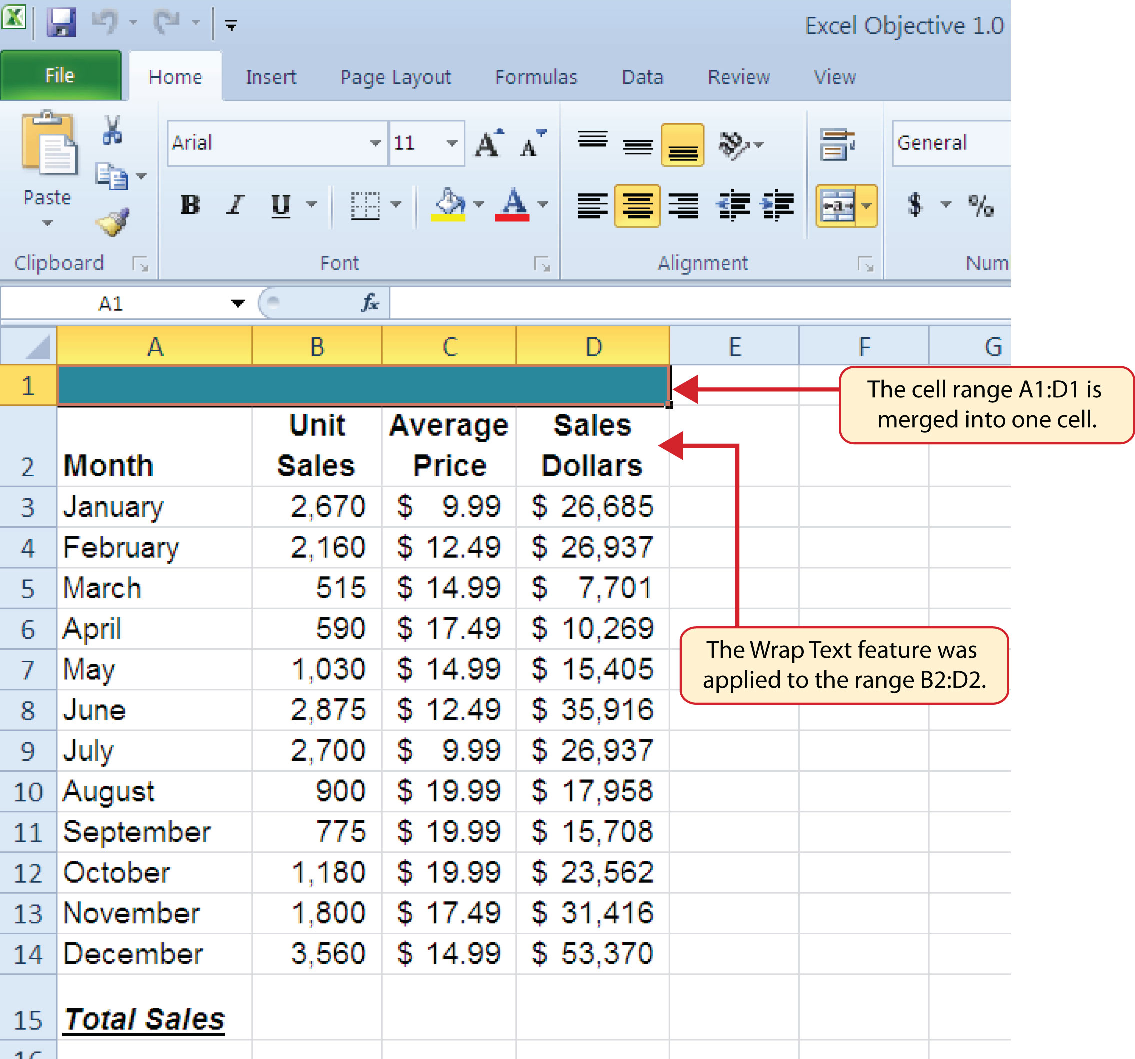
The skills presented in this segment show how data are aligned within cell locations. For example, text and numbers can be centered in a cell location, left justified, right justified, and so on. In some cases you may want to stack multiword text entries vertically in a cell instead of expanding the width of a column. This is referred to as wrapping textStacking multiword text entries vertically in a cell.. These skills are demonstrated in the following steps:
- Highlight the range B2:D2 by placing the mouse pointer over cell B2 and left clicking and dragging over to cell D2.
-
Click the Center button in the Alignment group of commands in the Home tab of the Ribbon (see Figure 1.40 "Alignment Group in Home Tab"). This will center the column headings in each cell location.
Figure 1.40 Alignment Group in Home Tab
-
Click the Wrap Text button in the Alignment group (see Figure 1.40 "Alignment Group in Home Tab"). The height of Row 2 automatically expands, and the words that were cut off because the columns were too narrow are now stacked vertically (see Figure 1.42 "Sheet1 with Data Alignment Features Added").
Mouseless Command
Wrap Text
- Press the ALT key and then the letters H and W one at a time.
Why?
Wrap Text
The benefit of using the Wrap Text command is that it significantly reduces the need to expand the column width to accommodate multiword column headings. The problem with increasing the column width is that you may reduce the amount of data that can fit on a piece of paper or one screen. This makes it cumbersome to analyze the data in the worksheet and could increase the time it takes to make a decision.
- Highlight the range A1:D1 by placing the mouse pointer over cell A1 and left clicking and dragging over to cell D1.
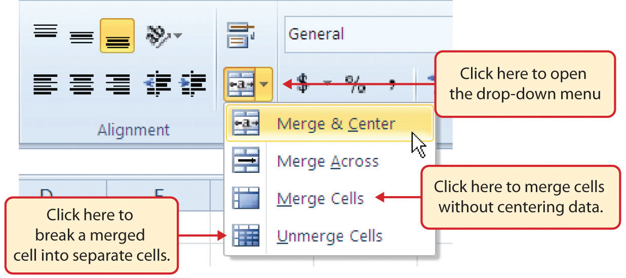
- Click the down arrow on the right side of the Merge & Center button in the Alignment group of commands in the Home tab of the Ribbon.
- Left click the Merge & Center option (see Figure 1.41 "Merge Cell Drop-Down Menu"). This will create one large cell location running across the top of the data set.
Mouseless Commands
Merge Commands
- Merge & Center: Press the ALT key and then the letters H, M, and C one at a time.
- Merge Cells: Press the ALT key and then the letters H, M, and M one at a time.
- Unmerge Cells: Press the ALT key and then the letters H, M, and U one at a time.
Figure 1.41 Merge Cell Drop-Down Menu
Why?
Merge & Center
One of the most common reasons the Merge & Center command is used is to center the title of a worksheet directly above the columns of data. Once the cells above the column headings are merged, a title can be centered above the columns of data. It is very difficult to center the title over the columns of data if the cells are not merged.
Figure 1.42 "Sheet1 with Data Alignment Features Added" shows the Sheet1 worksheet with the data alignment commands applied. The reason for merging the cells in the range A1:D1 will become apparent in the next segment.
Figure 1.42 Sheet1 with Data Alignment Features Added
Skill Refresher: Wrap Text
- Activate the cell or range of cells that contain text data.
- Click the Home tab of the Ribbon.
- Click the Wrap Text button.
Skill Refresher: Merge Cells
- Highlight a range of cells that will be merged.
- Click the Home tab of the Ribbon.
- Click the down arrow next to the Merge & Center button.
- Select an option from the Merge & Center list.
Entering Multiple Lines of Text
Follow-along file: Excel Objective 1.0 (Use file Excel Objective 1.07 if you are starting with this skill.)
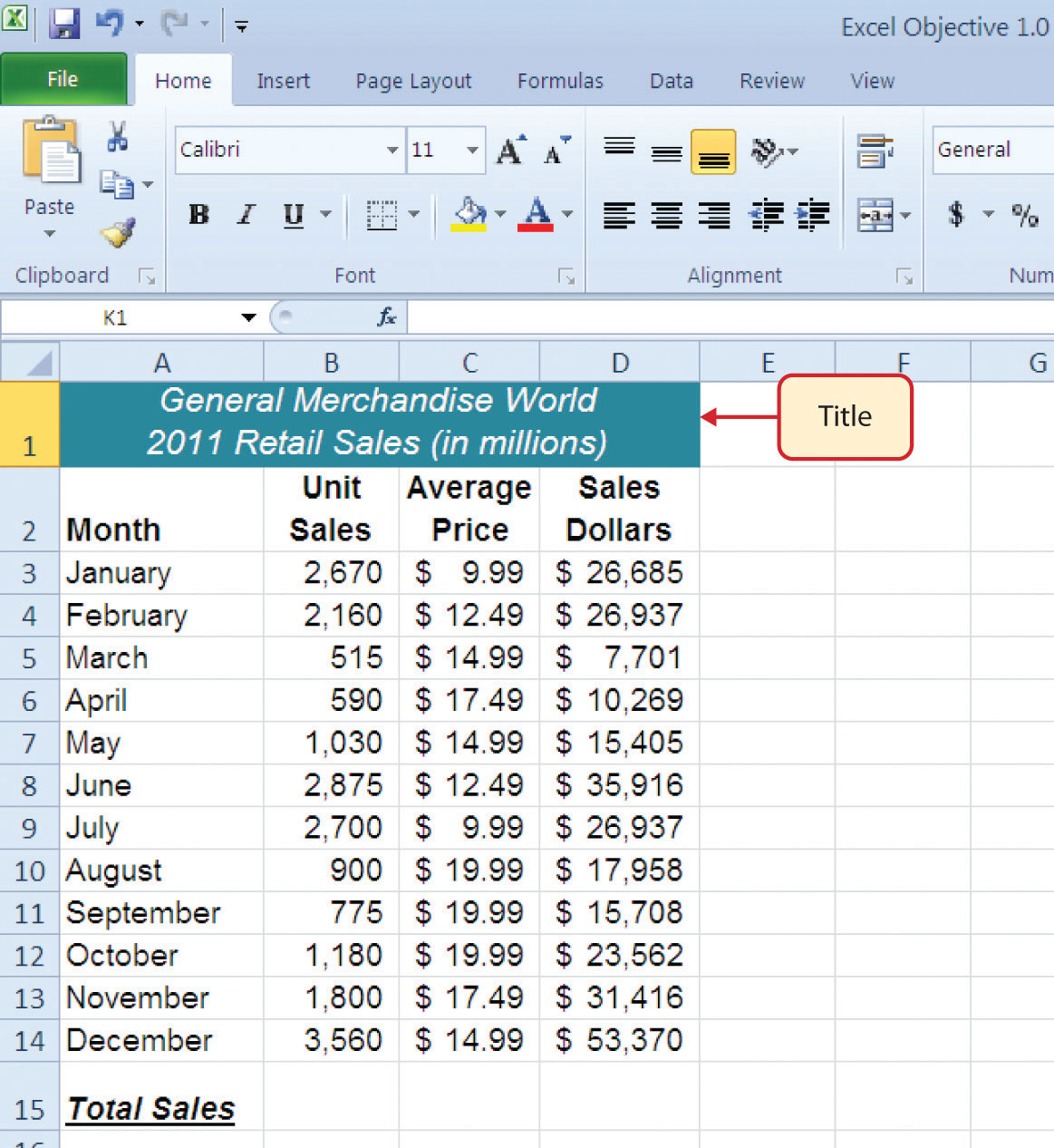
In the Sheet1 worksheet, the cells in the range A1:D1 were merged for the purposes of adding a title to the worksheet. This title will require that two lines of text be entered into a cell. The following steps explain how you can enter text into a cell and determine where you want the second line of text to begin:
- Activate cell A1 in the Sheet1 worksheet by placing the mouse pointer over cell A1 and clicking the left mouse button. Since the cells were merged, clicking cell A1 will automatically activate the range A1:D1.
- Type the text General Merchandise World.
- Hold down the ALT key and press the ENTER key. This will start a new line of text in this cell location.
- Type the text 2011 Retail Sales (in millions) and press the ENTER key.
- Select cell A1. Then click the Italics button in the Font group of commands in the Home tab of the Ribbon.
- Increase the height of Row 1 to 30 points. Once the row height is increased, all the text typed into the cell will be visible (see Figure 1.43 "Title Added to the Sheet1 Worksheet").
Figure 1.43 Title Added to the Sheet1 Worksheet
Skill Refresher: Entering Multiple Lines of Text
- Activate a cell location.
- Type the first line of text.
- Hold down the ALT key and press the ENTER key.
- Type the second line of text and press the ENTER key.
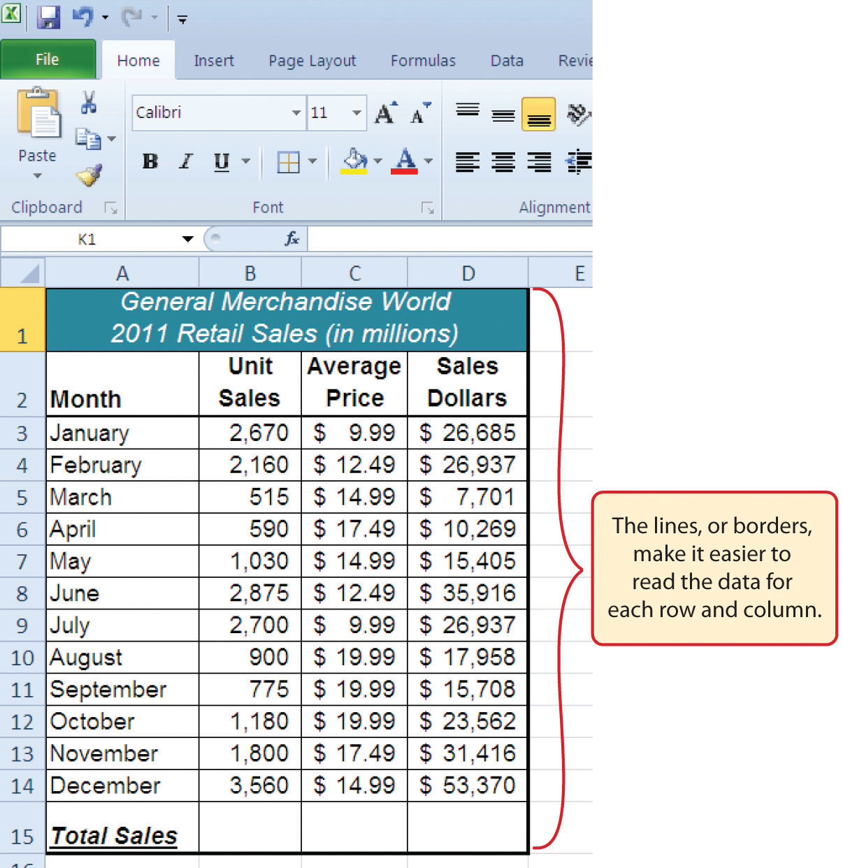
Borders (Adding Lines to a Worksheet)
Follow-along file: Excel Objective 1.0 (Use file Excel Objective 1.08 if you are starting with this skill.)
In Excel, adding custom lines to a worksheet is known as adding borders. BordersLines that are added to a worksheet to separate the data in columns and rows. are different from the grid lines that appear on a worksheet and that define the perimeter of the cell locations. The Borders command lets you add a variety of line styles to a worksheet that can make reading the worksheet much easier. The following steps illustrate methods for adding preset borders and custom borders to a worksheet:
- Note that when you click on cell A1, cells B1:D1 will also activate since they are merged.
-
Click the down arrow to the right of the Borders button in the Font group of commands in the Home page of the Ribbon (see Figure 1.44 "Borders Drop-Down Menu").
Figure 1.44 Borders Drop-Down Menu
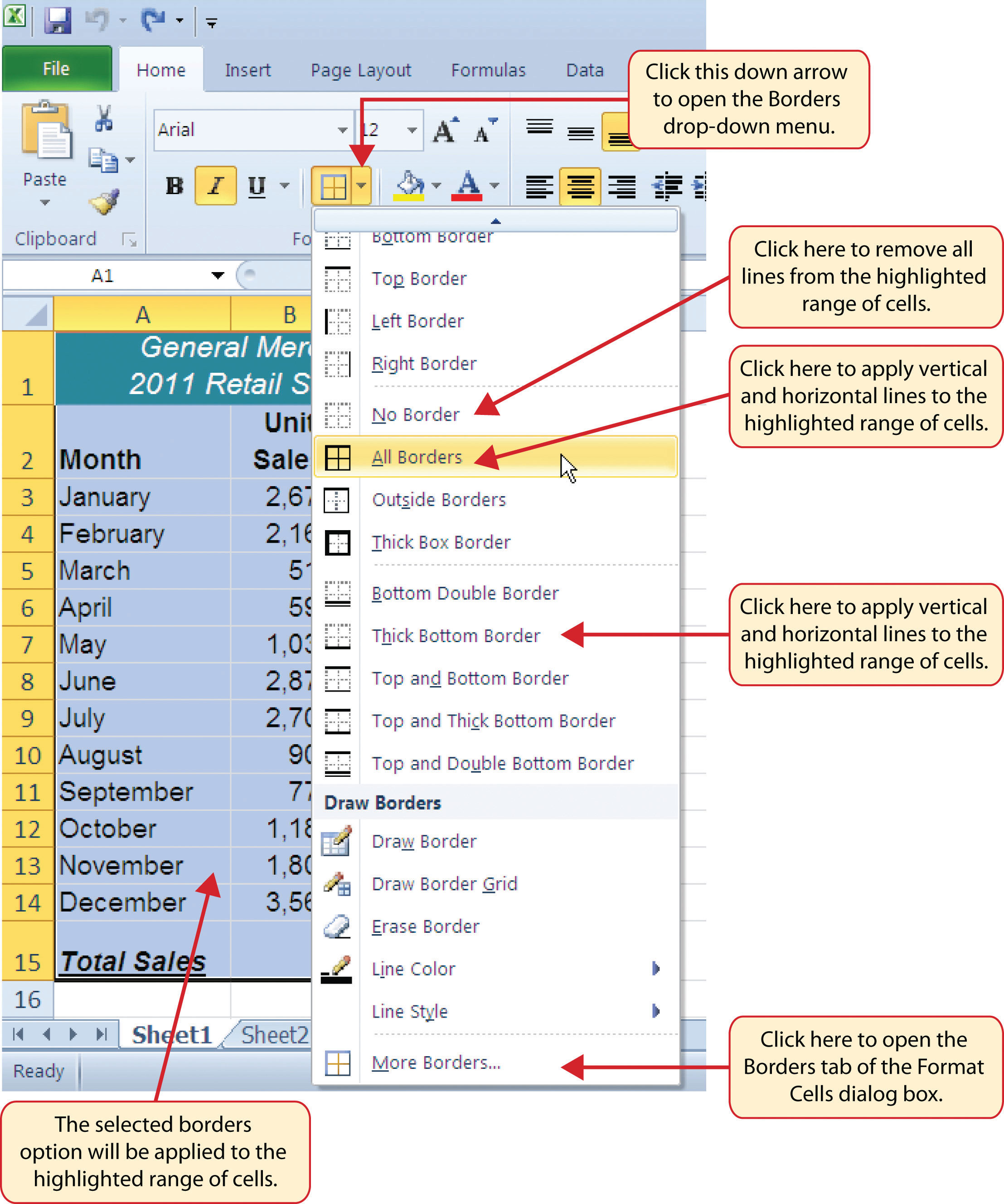
- Left click the All Borders option from the Borders drop-down menu (see Figure 1.44 "Borders Drop-Down Menu"). This will add vertical and horizontal lines to the range A1:D15.
- Highlight the range A2:D2 by placing the mouse pointer over cell A2 and left clicking and dragging over to cell D2.
- Click the down arrow to the right of the Borders button.
- Left click the Thick Bottom Border option from the Borders drop-down menu.
- Highlight the range A1:D15.
- Click the down arrow to the right of the Borders button.
- This will open the Format Cells dialog box (see Figure 1.45 "Borders Tab of the Format Cells Dialog Box"). You can access all formatting commands in Excel through this dialog box.
- In the Style section of the Borders tab, left click the thickest line style (see Figure 1.45 "Borders Tab of the Format Cells Dialog Box").
- Left click the Outline button in the Presets section (see Figure 1.45 "Borders Tab of the Format Cells Dialog Box").
- Click the OK button at the bottom of the dialog box (see Figure 1.45 "Borders Tab of the Format Cells Dialog Box").
Figure 1.45 Borders Tab of the Format Cells Dialog Box
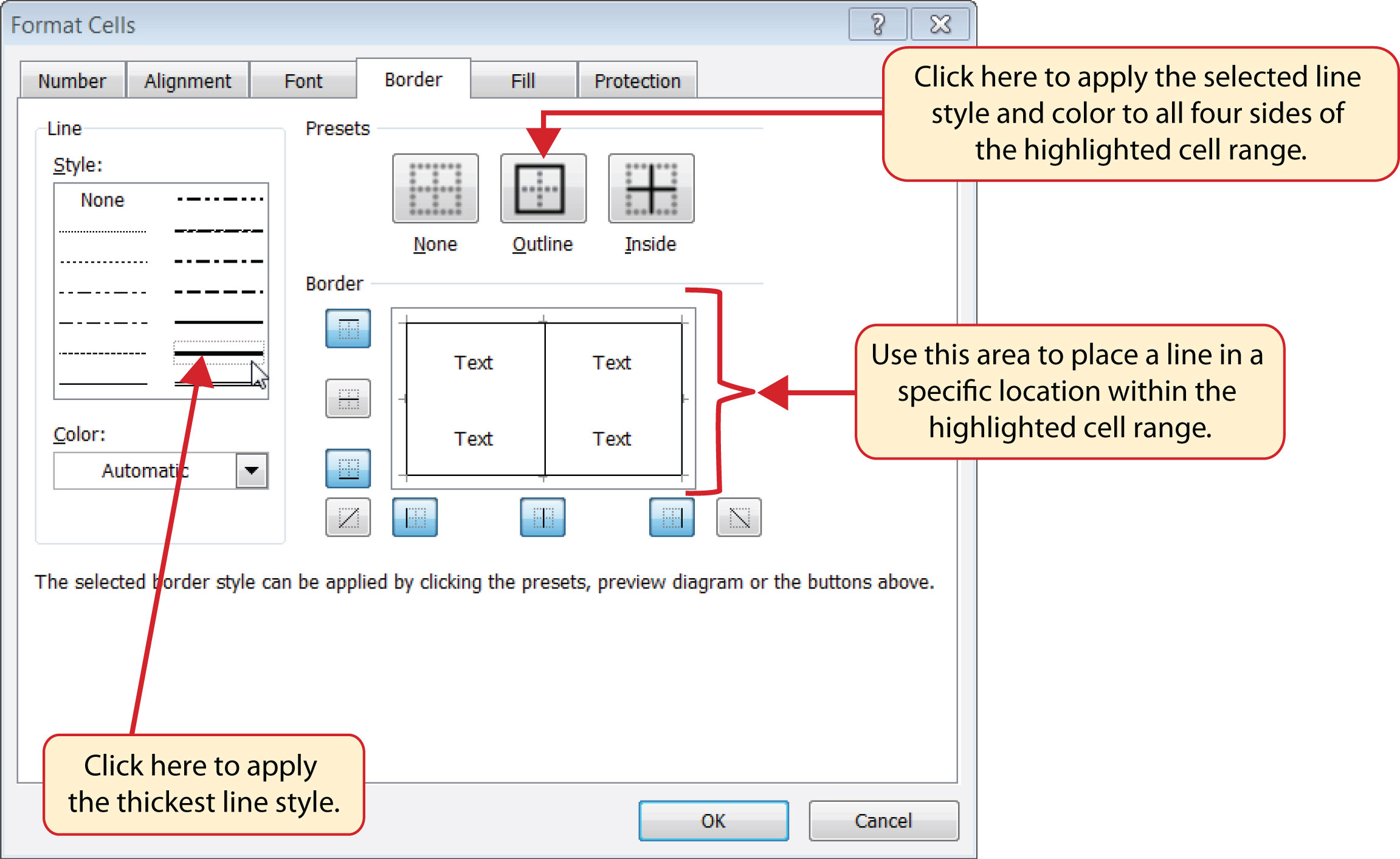
Figure 1.46 Borders Added to the Sheet1 Worksheet
Skill Refresher: Preset Borders
- Highlight a range of cells that require borders.
- Click the Home tab of the Ribbon.
- Click the down arrow next to the Borders button.
- Select an option from the preset borders list.
Skill Refresher: Custom Borders
- Highlight a range of cells that require borders.
- Click the Home tab of the Ribbon.
- Click the down arrow next to the Borders button.
- Select the More Borders option at the bottom of the options list.
- Select a line style and line color.
- Select a placement option.
- Click the OK button on the dialog box.
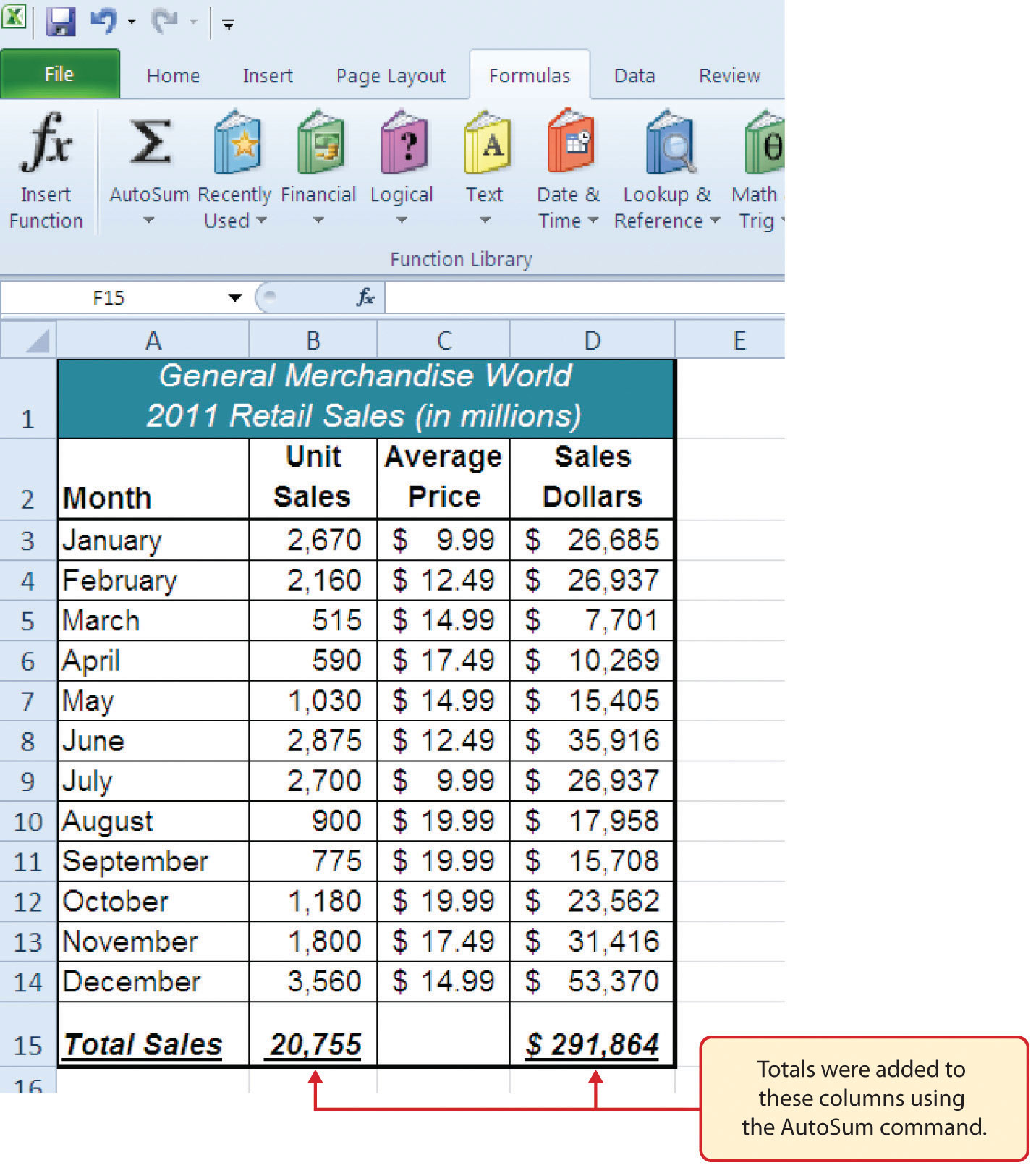
AutoSum
Follow-along file: Excel Objective 1.0 (Use file Excel Objective 1.09 if you are starting with this skill.)
You will see at the bottom of Figure 1.46 "Borders Added to the Sheet1 Worksheet" that Row 15 is intended to show the totals for the data in this worksheet. Applying mathematical computations to a range of cells is accomplished through functionsMathematical computations that are applied to a range of cells or specific cells on a worksheet. in Excel. Chapter 2 "Mathematical Computations" will review mathematical formulas and functions in detail. However, the following steps will demonstrate how you can quickly sum the values in a column of data using the AutoSum command:
- Activate cell B15 in the Sheet1 worksheet.
- Click the Formulas tab of the Ribbon.
-
Click the down arrow below the AutoSum button in the Function Library group of commands (see Figure 1.47 "AutoSum Drop-Down List"). Note that the AutoSum button can also be found in the Editing group of commands in the Home tab of the Ribbon.
Figure 1.47 AutoSum Drop-Down List
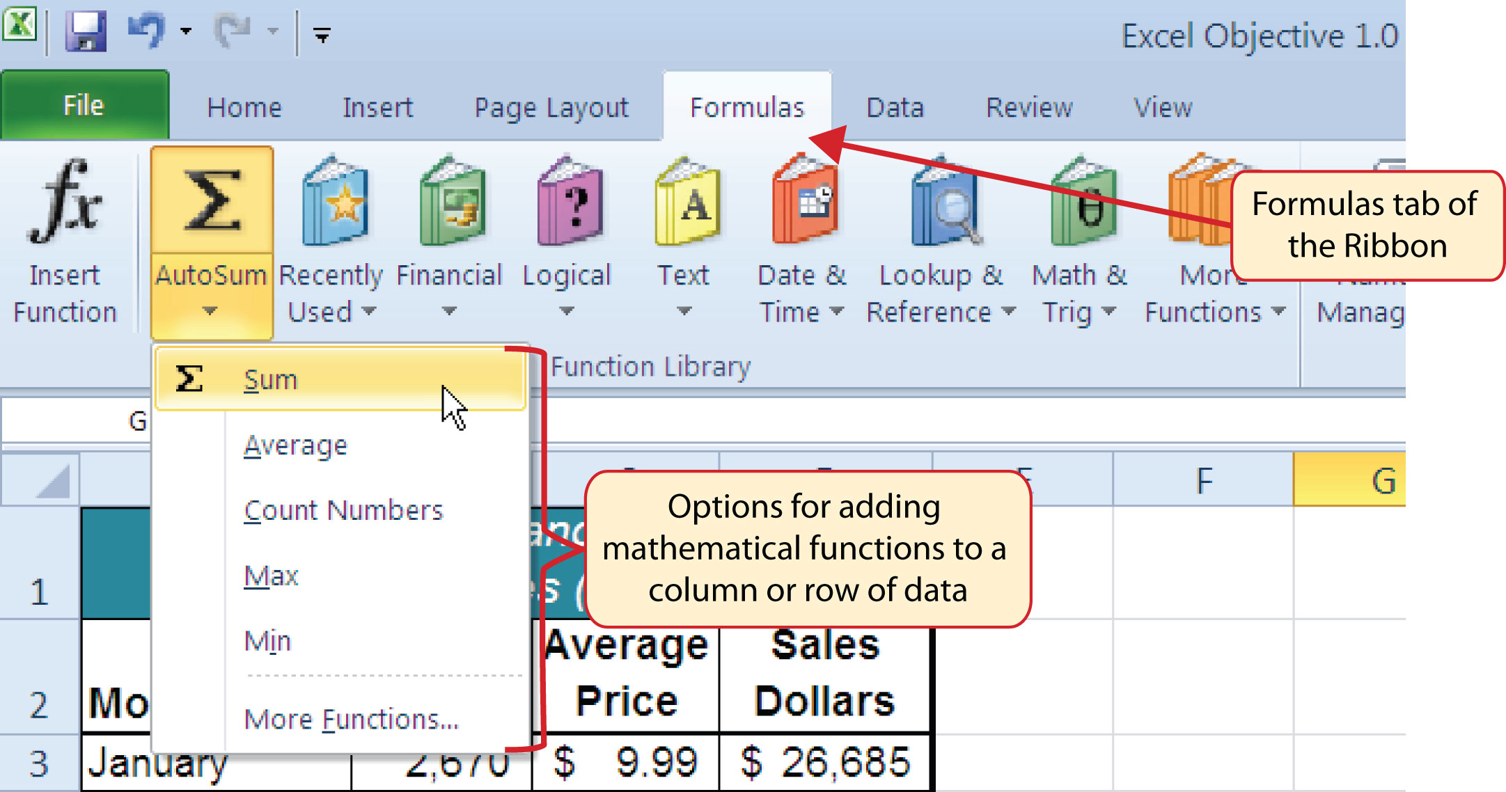
- Click the Sum option from the AutoSum drop-down menu.
- Excel will provide a total for the values in the Unit Sales column.
- Activate cell D15.
- Repeat steps 3 through 5 to sum the values in the Sales Dollars column (see Figure 1.48 "Totals Added to the Sheet1 Worksheet").
- This will remove the pound signs (####) and show the total.
Figure 1.48 Totals Added to the Sheet1 Worksheet
Skill Refresher: AutoSum
- Highlight a cell location below or to the right of a range of cells that contain numeric values.
- Click the Formulas tab of the Ribbon.
- Click the down arrow below the AutoSum button.
- Select a mathematical function from the list.
Inserting a Column Chart
Follow-along file: Excel Objective 1.0 (Use file Excel Objective 1.10 if you are starting with this skill.)
As mentioned at the beginning of this chapter, Excel serves as a critical tool for making decisions in both personal and professional contexts. ChartsTools used to graphically display the data in a worksheet. are a powerful tool in Excel that allow you to graphically display the data in a worksheet. Graphical displays allow the reader to immediately identify key trends and behaviors in the data that is being analyzed. For the workbook that we are using for this chapter, understanding the trends in monthly sales data is critical for making decisions such as how many staff members to assign to the store for each month as well as supplying the store with enough inventory to accommodate expected sales. To assist the reader in analyzing this data, a column chart will be created to graphically display the data. It is important for you to plan which type of chart will best display the data so your readers can quickly see key trends. More details on creating charts and on chart types will be presented in a later chapter. The following steps are an introduction to creating the column chart required for this chapter’s objective:
- Highlight the range A2:B14.
- Click the Insert tab of the Ribbon.
-
Click the Column button (see Figure 1.49 "Column Chart Drop-Down Menu"). This will open the column chart drop-down menu of options.
Figure 1.49 Column Chart Drop-Down Menu
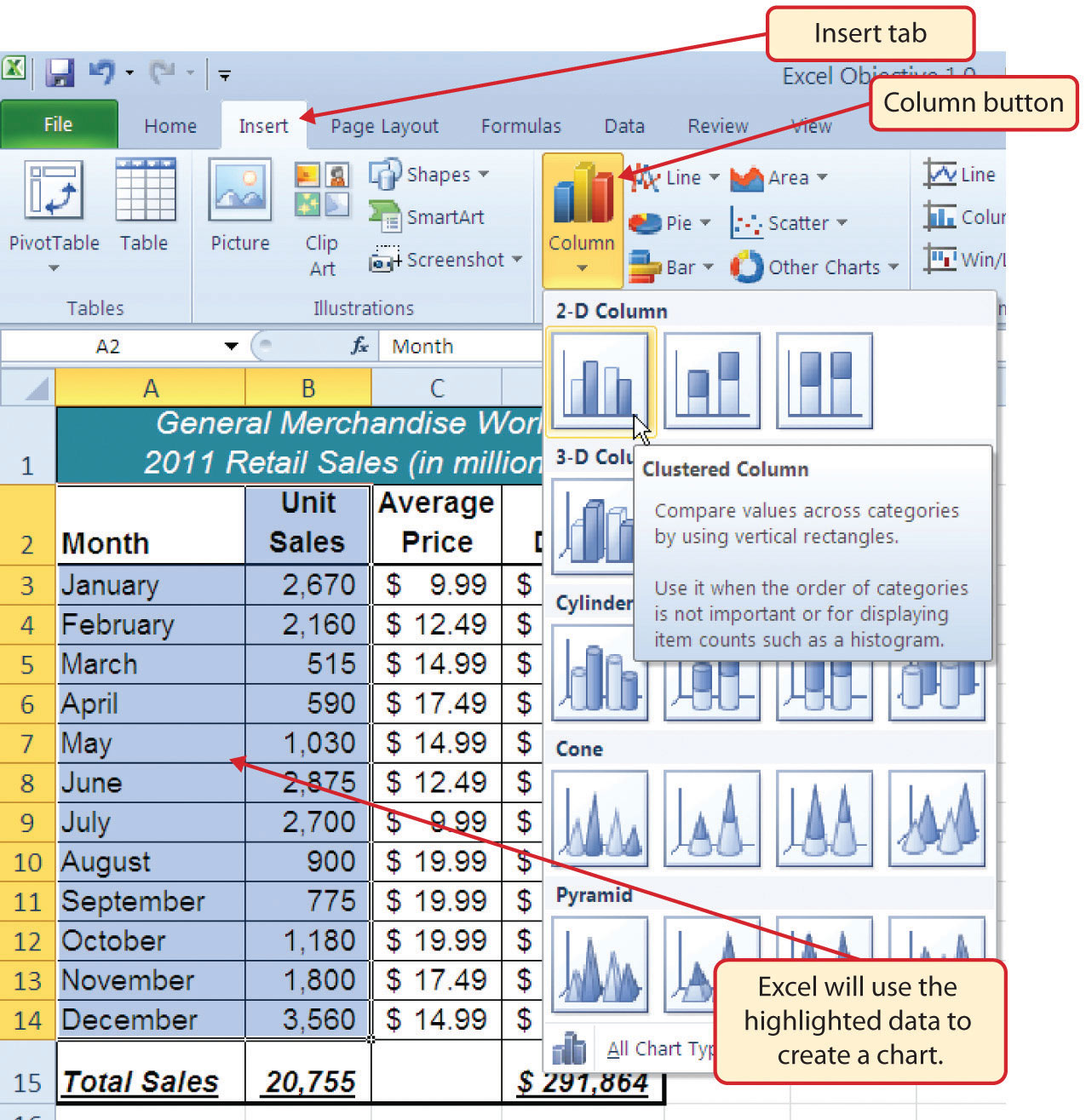
-
Select the Clustered Column option from the list of column chart options (see Figure 1.49 "Column Chart Drop-Down Menu"). This will create an embedded chart in the Sheet1 worksheet (see Figure 1.50 "Embedded Column Chart in Sheet1").
Figure 1.50 "Embedded Column Chart in Sheet1" shows the column chart that is created once a selection is made from the column chart drop-down menu. Notice that there are three new tabs added to the Ribbon. These tabs contain features for enhancing the appearance and construction of Excel charts. These commands will be covered in more detail in a later chapter. For now, you will see that Excel places the chart over the data in the worksheet. The following steps explain how to move and resize the chart:
Figure 1.50 Embedded Column Chart in Sheet1
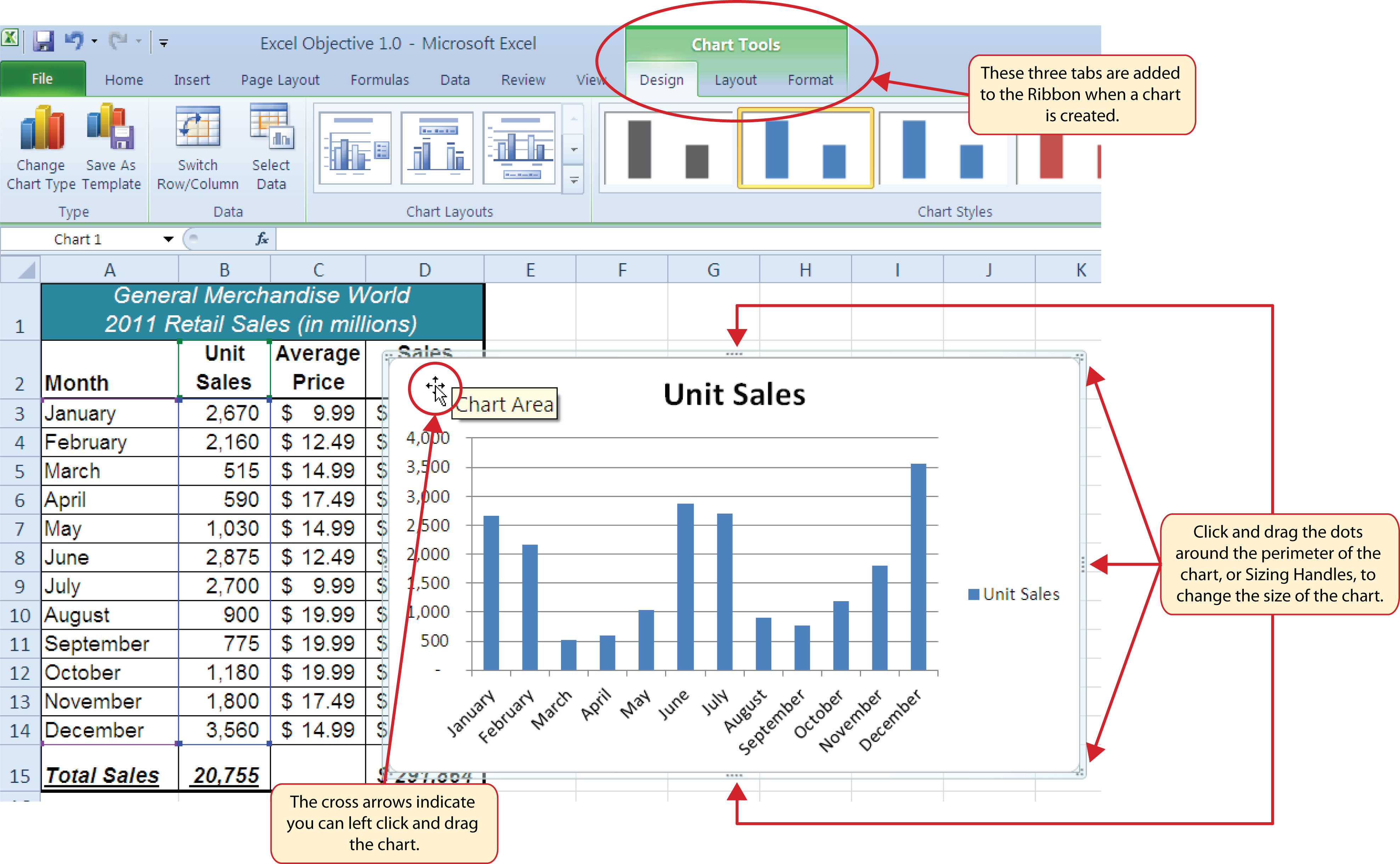
- The block white plus sign will become black cross arrows (see Figure 1.50 "Embedded Column Chart in Sheet1").
-
Left click and drag the chart so the upper left corner is placed in the middle of cell F1 (see Figure 1.51 "Moving an Embedded Chart").
Figure 1.51 Moving an Embedded Chart
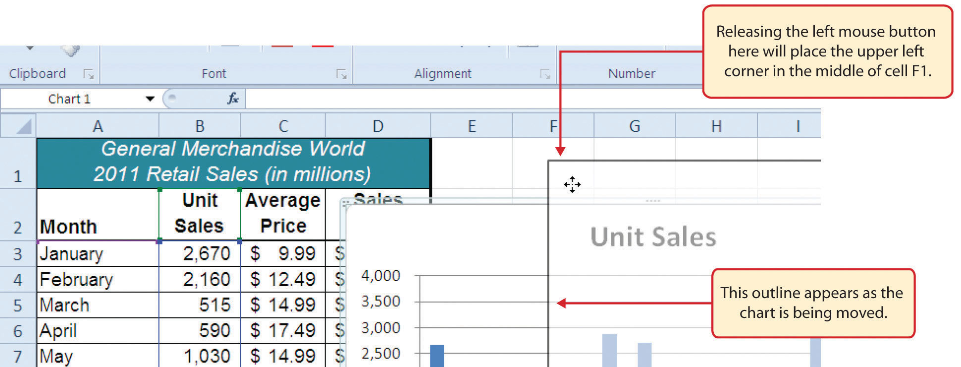
- Place the mouse pointer over the top center sizing handleDots that appear around the perimeter of an embedded chart in a worksheet. They can be clicked and dragged to desired dimensions to change the size of a chart. (see Figure 1.50 "Embedded Column Chart in Sheet1"). You will see the mouse pointer change from a white block plus sign to a vertical double arrow. Make sure the mouse pointer is not in the cross arrow mode as shown in Figure 1.50 "Embedded Column Chart in Sheet1" as this will move the chart instead of resizing it.
- While holding down the ALT key on your keyboard, left click and drag the mouse pointer slightly up. The chart will automatically adjust up to the top of Row 1.
- Place the mouse pointer over the left center sizing handle.
- While holding down the ALT key on your keyboard, left click and drag the mouse slightly toward the left. The chart will automatically adjust to the left side of Column F.
- Place the mouse pointer over the lower center sizing handle.
- While holding down the ALT key on your keyboard, left click and drag the mouse slightly down. The chart will automatically adjust to the bottom of Row 14.
- Place the mouse pointer over the right center sizing handle.
-
While holding down the ALT key on your keyboard, left click and drag the mouse slightly to the right. The chart will automatically adjust to the right side of Column M.
Why?
There Are No Sizing Handles on a Chart
If you do not see the dots or sizing handles around the perimeter of a chart, it could be that the chart is not activated. To activate a chart, left click anywhere on the chart.
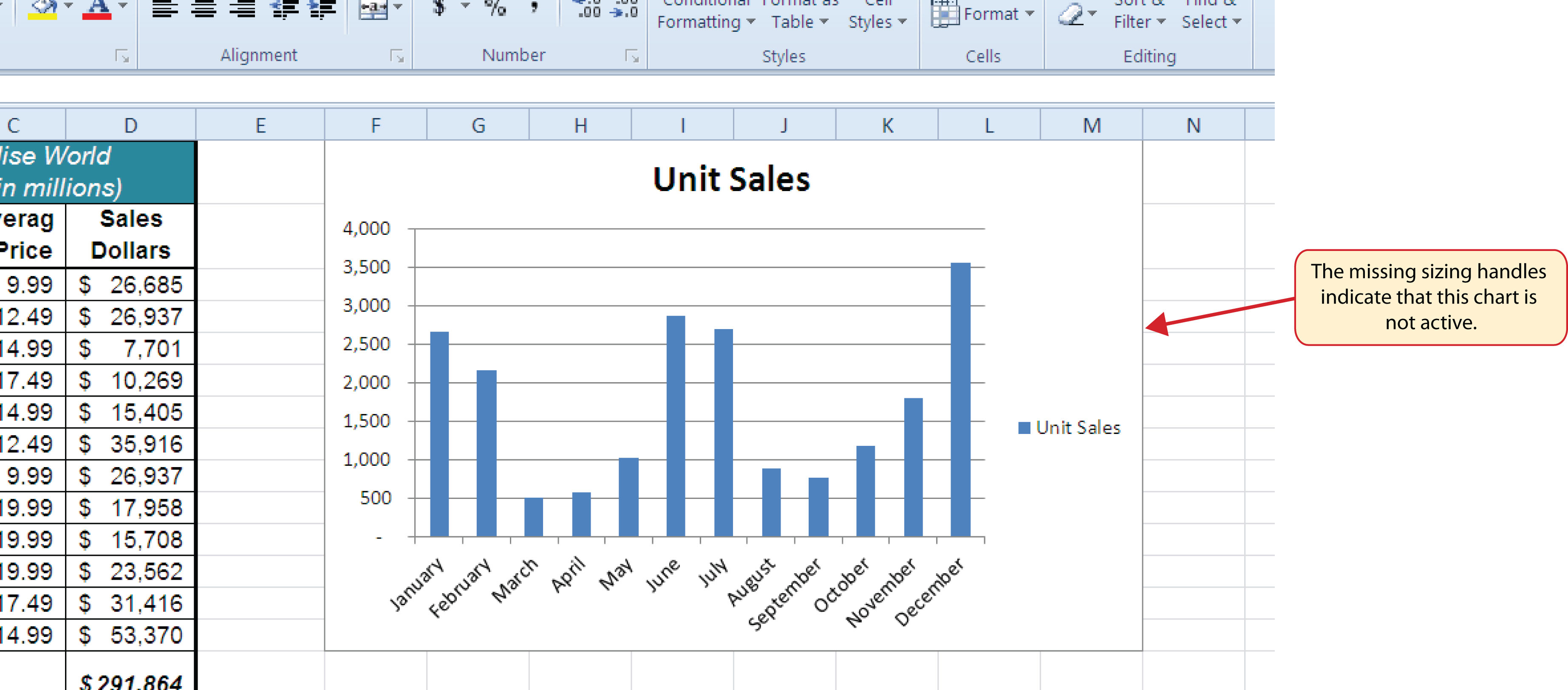
Figure 1.52 "Embedded Chart Moved and Resized" shows the column chart moved and resized. Notice that the sizing handles are not visible around the perimeter of the chart. This is because the chart is not activated. Once you click anywhere on the worksheet outside the chart area, the chart is automatically deactivated.
Figure 1.52 Embedded Chart Moved and Resized
Why?
Use the ALT Key When Resizing a Chart
Using the ALT key while resizing an embedded chart locks the perimeter of the chart to the columns and rows of the worksheet. This gives you the ability to adjust the chart to precise sizes as you adjust the width and height of the worksheet rows and columns.
As shown in Figure 1.50 "Embedded Column Chart in Sheet1", when a chart is created, three tabs are added to the Ribbon. The following steps explain how to use a few of the formatting and design features in these tabs:
- Check to make sure the column chart in Sheet1 is activated. To activate the chart, left click anywhere on the chart.
- Click the Design tab under the Chart Tools set of tabs on the Ribbon.
-
Click the down arrow on the right side of the Chart Styles section (see Figure 1.53 "Chart Styles in the Design Tab").
Figure 1.53 Chart Styles in the Design Tab
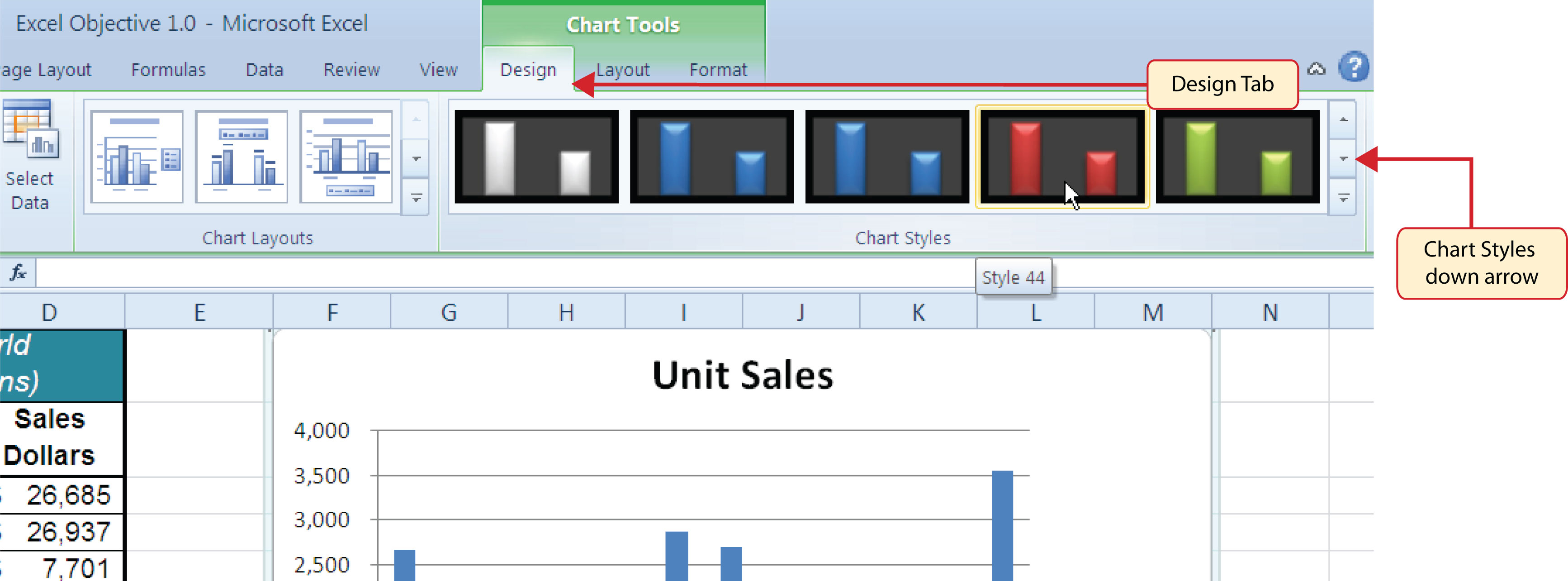
- Click Style 44 in the Chart Styles section. This style has a black background with red columns (see Figure 1.53 "Chart Styles in the Design Tab").
- Click the Format tab under the Chart Tools set of tabs on the Ribbon.
- Click the down arrow on the right side of the WordArt Styles section (see Figure 1.54 "WordArt Styles in the Format Tab").
Figure 1.54 WordArt Styles in the Format Tab
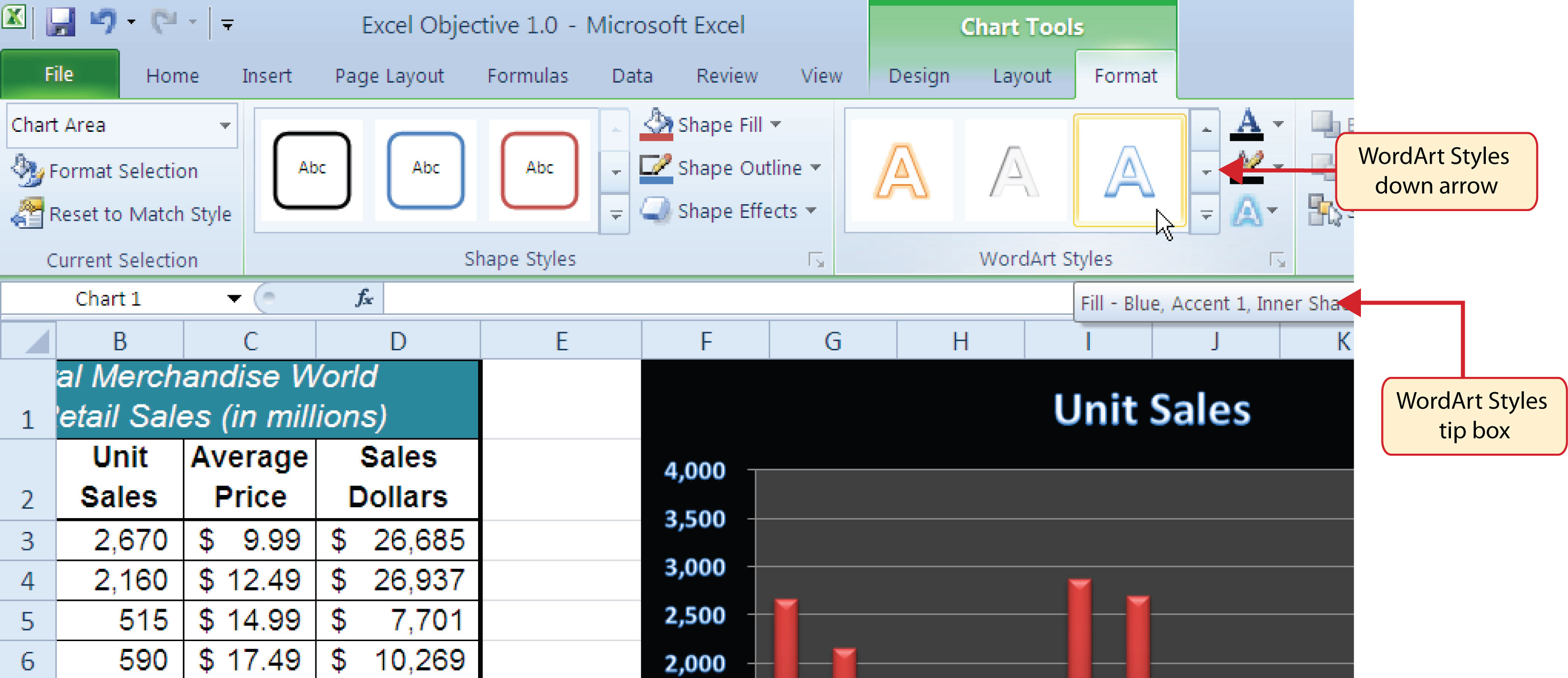
Click the Blue, Accent 1, Inner Shadow option (see Figure 1.54 "WordArt Styles in the Format Tab"). Notice that as you move the mouse pointer over the WordArt Styles options, the format of the chart title as well as the X and Y axis titles changes.
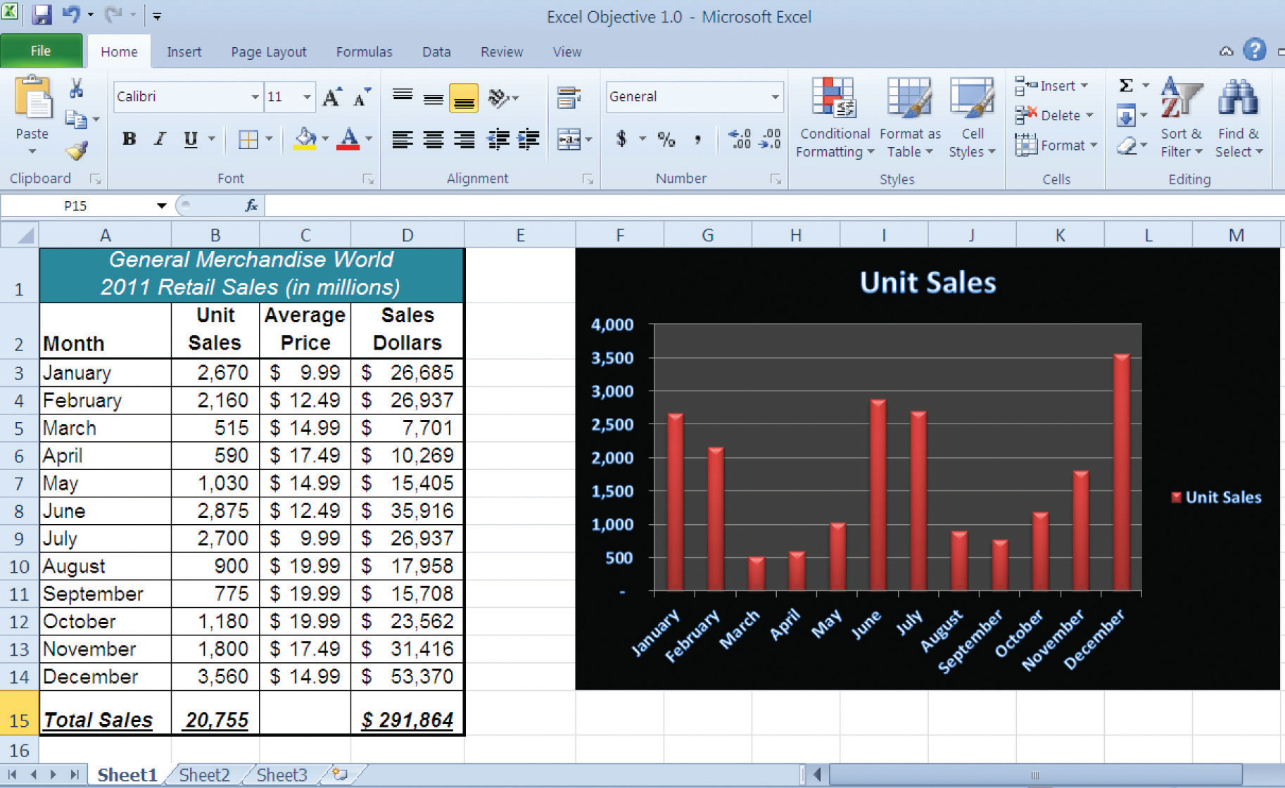
Figure 1.55 "Formatting Features Applied to the Column Chart" shows the embedded column chart with the formatting features applied. This chart is very effective in displaying the Unit Sales trends for this company. You can see very quickly that the tallest bar in the chart is the month of December, followed by the months of June, July, January, and February.
Figure 1.55 Formatting Features Applied to the Column Chart
Skill Refresher: Creating a Column Chart
- Highlight a range of cells that contain data that will be used to create the chart.
- Click the Insert tab of the Ribbon.
- Click the Column button in the Charts group.
- Select an option from the Column drop-down menu.
Cut, Copy, and Paste
Follow-along file: Excel Objective 1.0 (Use file Excel Objective 1.11 if you are starting with this skill.)
The Cut, Copy, and Paste commands are perhaps the most widely used commands in Microsoft Office. With regard to Excel, the Copy and Paste commands are often used to make copies of worksheets for developing different scenarios or versions for the data being analyzed. The following steps demonstrate how these commands are used for the objective in this chapter:
-
Click the Select All button in the upper left corner of the Sheet1 worksheet (see Figure 1.56 "Clipboard Group of Commands").
Figure 1.56 Clipboard Group of Commands
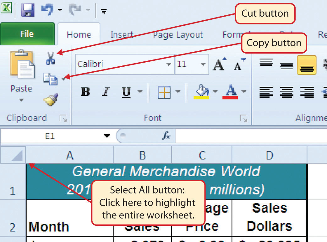
-
Click the Copy button in the Clipboard group of commands in the Home tab of the Ribbon (see Figure 1.56 "Clipboard Group of Commands").
Mouseless Command
Copy
- Press the CTRL key and then the letter C key on your keyboard.
- Open the Sheet2 worksheet by left clicking on the Sheet2 worksheet tab at the bottom of the workbook.
- Activate cell location A1.
-
Click the Paste button in the Clipboard group of commands in the Home tab of the Ribbon. Be sure to click the upper area of the Paste button and not the down arrow at the bottom of the button. A copy of Sheet1 will now appear in Sheet2.
Mouseless Command
Paste
- Press the CTRL key and then the letter V key on your keyboard.
- Click anywhere on the chart in the Sheet2 worksheet.
-
Click the Cut button in the Clipboard group on the Home tab of the Ribbon. This will remove the chart from the Sheet2 worksheet.
Mouseless Command
Cut
- Press the CTRL key and then the letter X key on your keyboard.
- Open the Sheet3 worksheet by left clicking on the Sheet3 worksheet tab at the bottom of the workbook.
- Activate cell location A1.
- Click the Paste button in the Home tab of the Ribbon. This will paste the chart from the Sheet2 worksheet into the Sheet3 worksheet.
Sorting Data (One Level)
Follow-along file: Excel Objective 1.0 (Use file Excel Objective 1.12 if you are starting with this skill.)
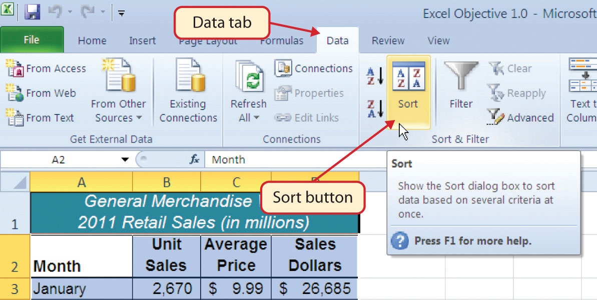
As mentioned earlier in this section, a chart is a tool that enables worksheet readers to analyze data quickly to spot key trends or patterns. Another powerful tool that provides similar benefits is the SortAn Excel command used to rank the data in a worksheet based on designated criteria. command. This feature ranks the rows of data in a worksheet based on designated criteria. The following steps demonstrate how the Sort command is used to rank the data in the Sheet2 worksheet:
- In the Sheet2 worksheet, highlight the range A2:D14.
- Click the Data tab of the Ribbon.
-
Click the Sort button in the Sort & Filter group of commands. This will open the Sort dialog box (see Figure 1.57 "Sort & Filter Group of Commands").
Figure 1.57 Sort & Filter Group of Commands
-
Click the down arrow next to the “Sort by” drop-down box in the Sort dialog box (see Figure 1.58 "Sort Dialog Box").
Figure 1.58 Sort Dialog Box
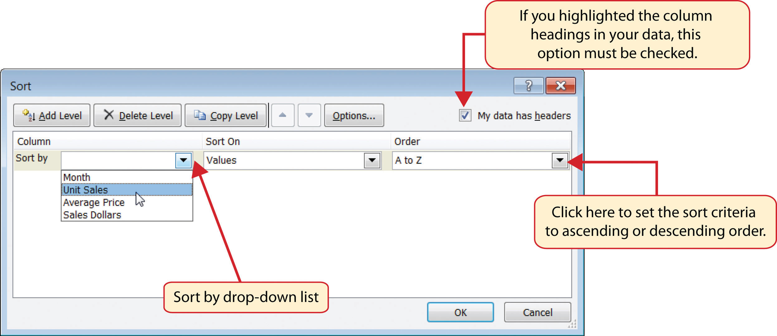
- Click the Unit Sales option from the drop-down list.
- Click the down arrow next to the Order drop-down box.
- Click Largest to Smallest from the drop-down list.
- Click the OK button at the bottom of the Sort dialog box. The data in the range A2:D14 will now be sorted in descending order based on the values in the Unit Sales column.
Integrity Check
Sorting Data
Carefully check the highlighted range of the data you are sorting. It is critical that all columns in a contiguous range of data are highlighted before sorting. If you do not sort all the columns in a data set, the data could become corrupted in such a way that it may not be corrected. If Excel detects that you are trying to sort only part of a contiguous range of data, it will give you a warning dialog box.
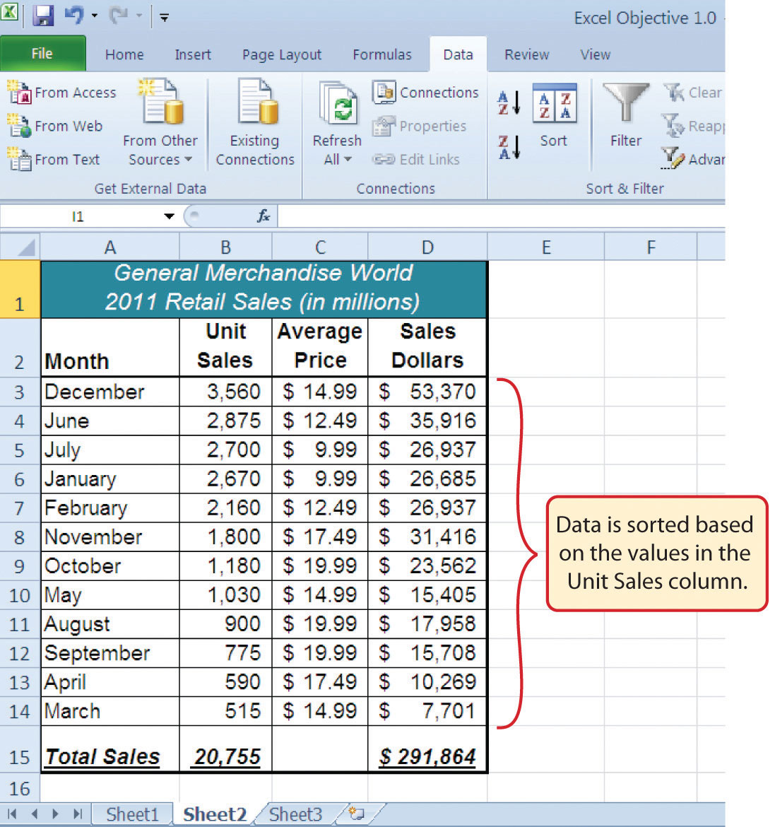
Figure 1.59 "Data Sorted Based on Unit Sales" shows the data in the Sheet2 worksheet sorted based on the values in the Unit Sales column. Similar to the chart, the Sort command makes it easy to identify the months of the year with the highest unit sales.
Figure 1.59 Data Sorted Based on Unit Sales
Skill Refresher: Sorting Data (One Level)
- Highlight a range of cells to be sorted.
- Click the Data tab of the Ribbon.
- Click the Sort button in the Sort & Filter group.
- Select a column from the “Sort by” drop-down list.
- Select a sort order from the Order drop-down list.
- Click the OK button on the Sort dialog box.
Moving, Renaming, Inserting, and Deleting Worksheets
Follow-along file: Excel Objective 1.0 (Use file Excel Objective 1.13 if you are starting with this skill.)
The default names for the worksheet tabs at the bottom of workbook are Sheet1, Sheet2, and so on. However, you can change the worksheet tab names to identify the data you are using in a workbook. Additionally, you can change the order in which the worksheet tabs appear in the workbook. The following steps explain how to rename and move the worksheets in a workbook:
- With the left mouse button, double click the Sheet1 worksheet tab at the bottom of the workbook (see Figure 1.60 "Renaming a Worksheet Tab").
- Type the name Sales by Month.
- Press the ENTER key on your keyboard.
- With the left mouse button, double click the Sheet2 worksheet tab at the bottom of the workbook.
- Type the name Unit Sales Rank.
-
Press the ENTER key on your keyboard.
Figure 1.60 Renaming a Worksheet Tab
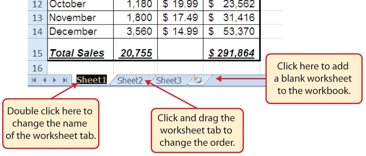
- Left click and drag the Unit Sales Rank worksheet tab to the left of the Sales by Month worksheet tab.
- Click the Sheet3 worksheet tab.
- Click the Home tab of the Ribbon.
- Click the down arrow on the Delete button in the Cells group of commands.
- Click the Delete Sheet option from the drop-down list (see Figure 1.35 "Delete Drop-Down Menu").
- Click the Delete button on the Delete warning box.
- Click the Insert Worksheet tab at the bottom of the workbook (see Figure 1.60 "Renaming a Worksheet Tab").
Integrity Check
Deleting Worksheets
Be very cautious when deleting worksheets that contain data. Once a worksheet is deleted, you cannot use the Undo command to bring the sheet back. Deleting a worksheet is a permanent command.
Mouseless Command
Inserting New Worksheets
- Press the SHIFT key and then the F11 key on your keyboard.
Figure 1.61 "Final Appearance of the Excel Objective 1.0 Workbook" shows the final appearance of the Excel Objective 1.0 workbook after the worksheet tabs have been renamed and moved.
Figure 1.61 Final Appearance of the Excel Objective 1.0 Workbook
Skill Refresher: Renaming Worksheets
- Double click the worksheet tab.
- Type the new name.
- Press the ENTER key.
Skill Refresher: Moving Worksheets
- Left click the worksheet tab.
- Drag it to the desired position.
Skill Refresher: Deleting Worksheets
- Open the worksheet to be deleted.
- Click the Home tab of the Ribbon.
- Click the down arrow on the Delete button.
- Select the Delete Sheet option.
- Click Delete on the warning box.
Key Takeaways
- Formatting skills are critical for creating worksheets that are easy to read and have a professional appearance.
- A series of pound signs (####) in a cell location indicates that the column is too narrow to display the number entered.
- Using the Wrap Text command allows you to stack multiword column headings vertically in a cell location, reducing the need to expand column widths.
- Use the Merge & Center command to center the title of a worksheet directly over the columns that contain data.
- Adding borders or lines will make your worksheet easier to read and helps to separate the data in each column and row.
- Effective charts enable readers to immediately identify key trends in the data you are displaying.
- Check to make sure all the data in a contiguous range of cells is highlighted before using the Sort command. Highlighting and sorting only part of a contiguous data set could corrupt your data in such a way that its integrity may not be restored.
- You cannot use the Undo command to bring back a worksheet that has been deleted.
Exercises
-
The pound signs (####) that appear in a cell location indicate that:
- A computational error has occurred.
- The AutoSum feature was applied to text data instead of numeric data.
- A number is too long for the current width of a column.
- You must click the Calculate Sheet command in the Formulas tab of the Ribbon.
-
Which of the following is most accurate with respect to the Wrap Text command?
- It allows you to designate which words are placed on a second line in a cell.
- It reduces the need to expand the width of the columns in a worksheet.
- It converts any numeric data to text data.
- It can be accessed only through the right-click menu of options.
-
What is the quickest way to center a title over six columns of data?
- Type the title into the cell location over the left-most column and use the space bar to try and place the title over the center of the six columns.
- Type the title into the cell location over the left-most column and click the Center alignment button in the Home tab of the Ribbon.
- Type the title into the cell location over the third column and use the BACKSPACE key to place the title over the center of the six columns.
- Highlight the six cell locations over each of the columns and click the Merge & Center button in the Home tab of the Ribbon.
-
Which of the following is true with respect to deleting worksheets?
- You cannot use the Undo button to bring back a worksheet once it has been deleted.
- Click the Select All button and press the DELETE key on your keyboard to delete a worksheet from a workbook.
- Holding down the SHIFT key while pressing the F11 key on your keyboard will delete a worksheet from your workbook.
- Excel will not let you delete a worksheet that contains data. All data must be removed from the worksheet before the worksheet can be deleted.
1.4 Printing
Learning Objectives
- Use the Page Layout tab to prepare a worksheet for printing.
- Add headers and footers to a printed worksheet.
- Examine how to print worksheets and workbooks.
Once you have completed a workbook, it is good practice to select the appropriate settings for printing. These settings are in the Page Layout tab of the Ribbon and discussed in this section of the chapter.
Page Setup
Follow-along file: Excel Objective 1.0 (Use file Excel Objective 1.14 if you are starting with this skill.)
Before you can properly print the worksheets in a workbook, you must establish appropriate settings. The following steps explain several of the commands in the Page Layout tab of the Ribbon used to prepare a worksheet for printing:
- Open the Unit Sales Rank worksheet by left clicking on the worksheet tab.
- Click the Page Layout tab of the Ribbon.
- Click the Margins button in the Page Setup group of commands. This will open a drop-down list of options for setting the margins of your printed document.
- Click the Wide option from the Margins drop-down list.
- Open the Sales by Month worksheet by left clicking on the worksheet tab.
- Click the Page Layout tab of the Ribbon (see Figure 1.62 "Page Layout Commands for Printing").
- Click the Margins button in the Page Setup group of commands.
- Click the Narrow option from the Margins drop-down list.
- Click the Orientation button in the Page Setup group of commands.
- Click the Landscape option.
- Click the down arrow to the right of the Width button in the Scale to Fit group of commands.
- Click the 1 Page option from the drop-down list.
- Click the down arrow to the right of the Height button in the Scale to Fit group of commands.
- Click the 1 Page option from the drop-down list. This step along with step 12 will automatically reduce the worksheet so that it fits on one piece of paper. It is very common for professionals to create worksheets that fit within the width of the paper being used. However, for long data sets, you may need to set the height to more than one page. Table 1.2 "Printing Resources: Purpose and Use for Page Setup Commands" provides a list of commands found in the Page Layout tab of the Ribbon
Why?
Use Print Settings
Because professionals often share Excel workbooks, it is a good practice to select the appropriate print settings in the Page Layout tab even if you do not intend to print the worksheets in a workbook. It can be extremely frustrating for recipients of a workbook who wish to print your worksheets to find that the necessary print settings have not been selected. This may reflect poorly on your attention to detail, especially if the recipient of the workbook is your boss.
Figure 1.62 Page Layout Commands for Printing
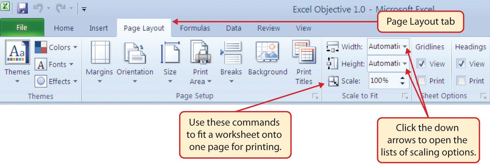
Table 1.2 Printing Resources: Purpose and Use for Page Setup Commands
| Command | Purpose | Use |
|---|---|---|
| Margins | Sets the top, bottom, right, and left margin space for the printed document | 1. Click the Page Layout tab of the Ribbon. |
| 2. Click the Margin button. | ||
| 3. Click one of the preset margin options or click Custom Margins. | ||
| Orientation | Sets the orientation of the printed document to either portrait or landscape | 1. Click the Page Layout tab of the Ribbon. |
| 2. Click the Orientation button. | ||
| 3. Click one of the preset orientation options. | ||
| Size | Sets the paper size for the printed document | 1. Click the Page Layout tab of the Ribbon. |
| 2. Click the Size button. | ||
| 3. Click one of the preset paper size options or click More Paper Sizes. | ||
| Print Area | Used for printing only a specific area or range of cells on a worksheet | 1. Highlight the range of cells on a worksheet that you wish to print. |
| 2. Click the Page Layout tab of the Ribbon. | ||
| 3. Click the Print Area button. | ||
| 4. Click the Set Print Area option from the drop-down list. | ||
| Breaks | Allows you to manually set the page breaks on a worksheet | 1. Activate a cell on the worksheet where the page break should be placed. Breaks are created above and to the left of the activated cell. |
| 2. Click the Page Layout tab of the Ribbon. | ||
| 3. Click the Breaks button. | ||
| 4. Click the Insert Page Break option from the drop-down list. | ||
| Background | Adds a picture behind the cell locations in a worksheet | 1. Click the Page Layout tab of the Ribbon. |
| 2. Click the Background button. | ||
| 3. Select a picture stored on your computer or network. | ||
| Print Titles | Used when printing large data sets that are several pages long. This command will repeat the column headings at the top of each printed page. | 1. Click the Page Layout tab of the Ribbon. |
| 2. Click the Print Titles button. | ||
| 3. Click in the Rows to Repeat at Top input box in the Page Setup dialog box. | ||
| 4. Click any cell in the row that contains the column headings for your worksheet. | ||
| 5. Click the OK button at the bottom of the Page Setup dialog box. |
Headers and Footers
Follow-along file: Excel Objective 1.0 (Use file Excel Objective 1.15 if you are starting with this skill.)
When printing worksheets from Excel, it is common to add headersSpace at the top of a printed worksheet that contains information such as the date, page number, file name, company name, and so on. and footersSpace at the bottom of a printed worksheet that contains information such as the date, page number, file name, company name, and so on. to the printed document. Information in the header or footer could include the date, page number, file name, company name, and so on. The following steps explain how to add headers and footers to the Excel Objective 1.0 workbook:
- Open the Unit Sales Rank worksheet by left clicking on the worksheet tab.
- Click the Insert tab of the Ribbon.
-
Click the Header & Footer button in the Text group of commands. You will see the Design tab added to the Ribbon; this is used for creating the headers and footers for the printed worksheet. Also, this will convert the view of the worksheet from Normal to Page Layout (see Figure 1.63 "Design Tab for Creating Headers and Footers").
Figure 1.63 Design Tab for Creating Headers and Footers
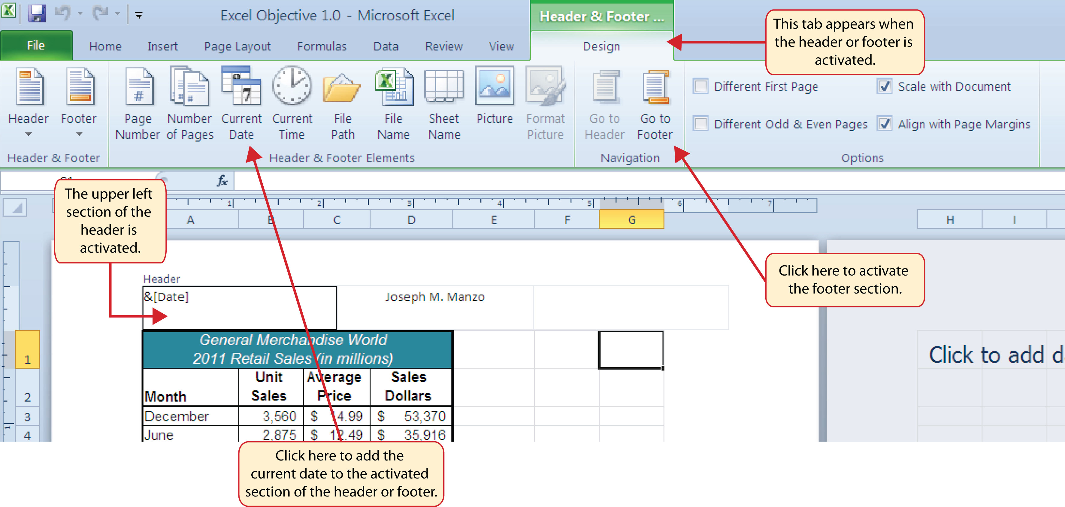
- Type your name in the center section of the Header.
- Place the mouse pointer over the left section of the Header and left click (see Figure 1.63 "Design Tab for Creating Headers and Footers").
- Click the Current Date button in the Header & Footer Elements group of commands in the Design tab of the Ribbon.
- Click the Go to Footer button in the Navigation group of commands in the Design tab of the Ribbon.
- Place the mouse pointer over the far right section of the footer and left click.
- Click the Page Number button in the Header & Footer Elements group of commands in the Design tab of the Ribbon.
- Click any cell location outside the header or footer area. The Design tab for creating headers and footers will disappear.
-
Click the Normal view button in the lower right side of the Status Bar (see Figure 1.64 "Worksheet in Page Layout View").
Figure 1.64 Worksheet in Page Layout View
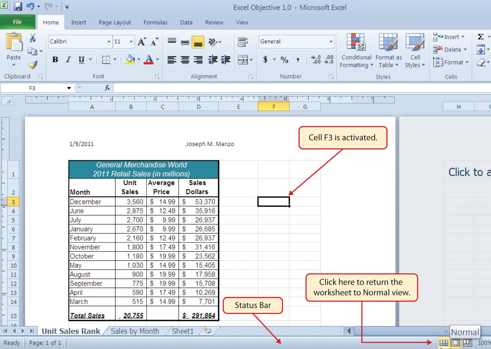
- Open the Sales by Month worksheet by left clicking the worksheet tab.
- Repeat steps 2 through 11 to create the same header and footer for this worksheet.
Printing Worksheets and Workbooks
Follow-along file: Excel Objective 1.0 (Use file Excel Objective 1.16 if you are starting with this skill.)
Once you have established the print settings for the worksheets in a workbook and have added headers and footers, you are ready to print your worksheets. The following steps explain how to print the worksheets in the Excel Objective 1.0 workbook:
- Open the Unit Sales Rank worksheet by left clicking on the worksheet tab.
- Click the File tab on the Ribbon.
-
Click the Print option on the left side of the Backstage view (see Figure 1.65 "Print Preview"). On the right side of the Backstage view, you will be able to see a preview of your printed worksheet.
Figure 1.65 Print Preview
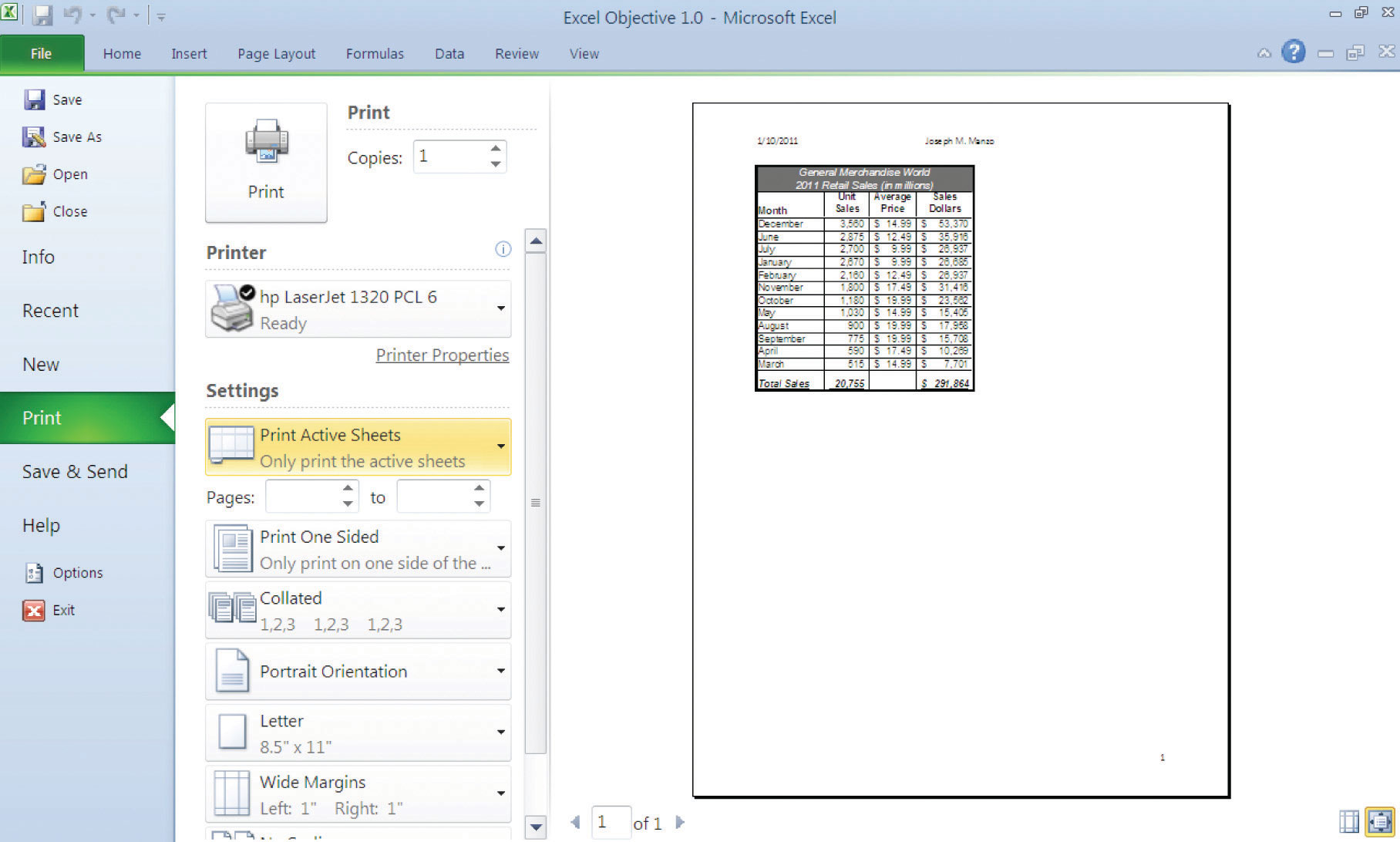
- Click the Print Active Sheets button in the Print section of the Backstage view (see Figure 1.65 "Print Preview").
- Click the Print Entire Workbook option from the drop-down list. This will print all worksheets in a workbook when the Print button is clicked.
- Click the Next Page arrow at the bottom of the preview window.
- Click the Print button.
- Click the Home tab of the Ribbon.
- Save and close the Excel Objective 1.0 workbook.
Key Takeaways
- The commands in the Page Layout tab of the Ribbon are used to prepare a worksheet for printing.
- You can add headers and footers to a worksheet to show key information such as page numbers, the date, the file name, your name, and so on.
- The Print commands are in the File tab of the Ribbon.
Exercises
-
Which of the following commands is used to print the column headings in a worksheet at the top of each printed page for a worksheet that contains 100 rows of data?
- the Header & Footer command in the Insert tab of the Ribbon
- the Print Titles command in the Page Layout tab of the Ribbon
- the Insert command in the Home tab of the Ribbon
- the Conditional Formatting command in the Home tab of the Ribbon
-
Which of the following is true with respect to printing Excel worksheets?
- Setting the Width and Height drop-down lists to 1 Page will ensure that all the worksheets in a workbook are printed on one page.
- The page layout settings must be set for each worksheet in a workbook.
- You can print only one worksheet at a time in a workbook that contains multiple worksheets.
- All of the above are true.
1.5 Chapter Assignments and Tests
To assess your understanding of the material covered in the chapter, please complete the following assignments.
Careers in Practice (Skills Review)
Basic Monthly Budget for Medical Office (Comprehensive Review)
Starter File: Chapter 1 CiP Exercise 1
Difficulty: Level 1
Creating and maintaining budgets are common practices in many careers. Budgets play a critical role in helping a business or household control expenditures. In this exercise you will create a budget for a hypothetical medical office while reviewing the skills covered in this chapter. Begin the exercise by opening the file named Chapter 1 CiP Exercise 1.
Entering, Editing, and Managing Data
- Activate all the cell locations in the Sheet1 worksheet by left clicking the Select All button in the upper left corner of the worksheet.
- In the Home tab of the Ribbon, set the font style to Arial and the font size to 12 points.
- Increase the width of Column A so all the entries in the range A3:A8 are visible. Place the mouse pointer between the letter A and letter B of Column A and Column B. When the mouse pointer changes to a double arrow, left click and drag it to the right until the character width is 18.00.
- Enter Quarter 1 in cell B2.
- Use AutoFill to complete the headings in the range C2:E2. Activate cell B2 and place the mouse pointer over the Fill Handle. When the mouse pointer changes to a black plus sign, left click and drag it to cell E2.
- Increase the width of Columns B, C, D, and E to 10.14 characters. Highlight the range B2:E2 and click the Format button in the Home tab of the Ribbon. Click the Column Width option, type 10.14 in the Column Width dialog box, and then click the OK button in the Column Width dialog box.
- Enter the words Medical Office Budget in cell A1.
- Insert a blank column between Columns A and B. Activate any cell location in Column B. Then, click the drop-down arrow of the Insert button in the Home tab of the Ribbon. Click the Insert Sheet Columns option.
- Enter the words Budget Cost in cell B2.
-
Adjust the width of Column B to 13.29 characters.
Formatting and Basic Charts
- Merge the cells in the range A1:F1. Highlight the range and click the Merge & Center button in the Home tab of the Ribbon.
- Make the following format adjustments to the range A1:F1: bold; italics; change the font size to 14 points; change the cell fill color to Aqua, Accent 5, Darker 50%; and change the font color to white.
- Increase the height of Row 1 to 24.75 points.
- Center the title of the worksheet in the range A1:F1 vertically. Activate the range and then click the Middle Align button in the Home tab of the Ribbon.
- Make the following format adjustment to the range A2:F2: bold; and change the cell fill color to Tan, Background 2, Darker 10%.
- Set the alignment in cell B2 to Wrap Text. Activate the cell location and click the Wrap Text button in the Home tab of the Ribbon.
- Copy cell C3 and paste the contents into the range D3:F3.
- Copy the contents in the range C6:C8 by highlighting the range and clicking the Copy button in the Home tab of the Ribbon. Then, highlight the range D6:F8 and click the Paste button in the Home tab of the Ribbon.
- Calculate the total budget for all four quarters for the salaries. Activate cell B3 and click the down arrow on the AutoSum button in the Formulas tab of the Ribbon. Click the Sum option from the drop-down list. Then, highlight the range C3:F3 and press the ENTER key on your keyboard.
- Copy the contents of cell B3 and paste them into the range B4:B8.
- Format the range B3:F8 with a US dollar sign and zero decimal places.
- Sort the data in the range A2:F8 based on the values in the Quarter 4 column in ascending order. Highlight the range A2:F8 and click the Sort button in the Data tab of the Ribbon. Select Quarter 4 in the “Sort by” drop-down box and select Smallest to Largest in the Order drop-down box. Click the OK button.
- Add vertical and horizontal lines to the range A1:F8. Highlight the range and click the down arrow next to the Borders button in the Home tab of the Ribbon. Select the All Borders option from the drop-down list.
- Change the name of the Sheet1 worksheet tab to “Budget.” Double click the worksheet tab, type the word Budget, and press the ENTER key.
- Insert a pie chart using the data in the range A2:B8. Highlight the range and click the Pie button in the Insert tab of the Ribbon. Click the first option on the list (the Pie option).
- Click and drag the chart so the upper left corner is in the center of cell H2.
-
Add labels to the chart by clicking the Layout 1 option from the Chart Layouts list in the Design tab of the Ribbon. Make sure the chart is activated by clicking it once before you look for the Layout 1 Chart Layout option.
Printing
- Change the orientation of the Budget worksheet so it prints landscape instead of portrait.
- Adjust the appropriate settings so the Budget worksheet prints on one piece of paper.
- Add a header to the Budget worksheet that shows the date in the upper left corner and your name in the center.
- Add a footer to the Budget worksheet that shows the page number in the lower right corner.
- Use the Save As command in the File tab of the Ribbon to save the workbook by adding your name in front of the current workbook name (i.e., “your name Chapter 1 CiP Exercise 1”).
- Close the workbook and Excel.
Figure 1.66 Completed Medical Budget Exercise
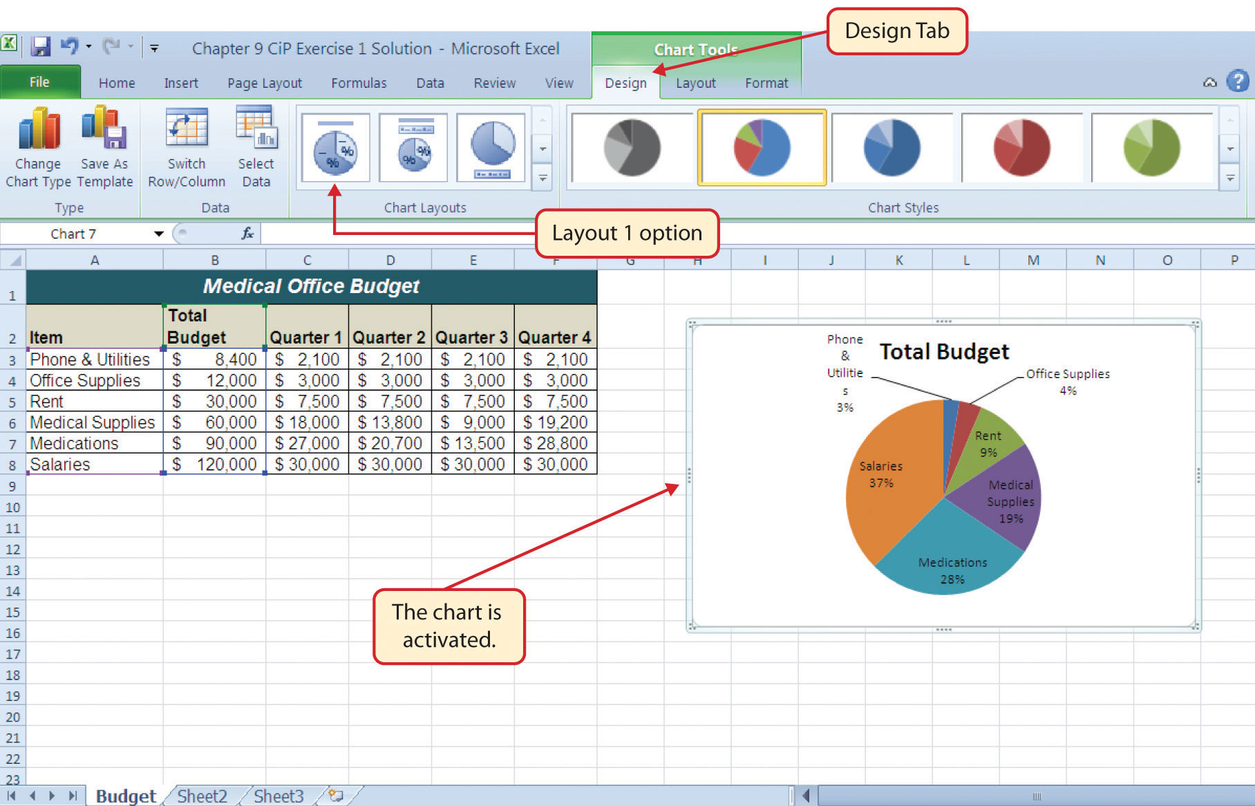
Marketing for Specialty Women’s Apparel
Starter File: Chapter 1 CiP Exercise 2
Difficulty: Level 2
A key activity for marketing professionals is to analyze how population demographics change in certain regions. This is especially important for specialty retail stores that target a specific age group within a population. This exercise utilizes the skills covered in this chapter to analyze hypothetical population trends. The decisions that can be made with such information include where to open new stores, whether existing stores should be closed and reopened in other communities, or whether the product assortment should be adjusted. The purpose of this exercise is to use the skills presented in this chapter to analyze hypothetical population trends for a fashion retailer.
- In the Sheet1 worksheet, enter the year 2008 into cell B3.
- Use AutoFill to fill the years 2009 to 2012 in the range C3:F3.
- Change the font style to Arial and the font size to 12 points for all cell locations in the Sheet1 worksheet.
- Merge and center the cells in the range A1:F1.
- Make the following formatting adjustments to the range A1:F1: bold; italics; change the cell fill color to Olive Green, Accent 3, Lighter 60%; change the font size to 14 points.
- Enter the title for this worksheet into the range A1:F1 on two lines. The first line should read Population Trends by Age Group. The second line should read for Region 5.
- Increase the height of Row 1 so the title is visible.
- Delete Row 2.
- Increase the height of Row 2 to 21 points.
- Format the values in the range B3:F6 so a comma separates each thousands place with zero decimal places.
- Make the necessary adjustments to remove any pound signs (####) that may have appeared after formatting the values.
- Sort the data in the range A2:F6 based on the values in the year 2008 from largest to smallest.
- Enter the word Totals in cell A7.
- Increase the height of Row 7 to 22.50 points.
- Format the range A7:F7 so entries are bold and italic.
- In cell B7, add a total that sums the values in the range B3:B6. Format the value with zero decimal places and a comma for each thousands place.
- Copy the contents of cell B7 and paste them into the range C7:F7.
- Add vertical and horizontal lines to the range A1:F7.
- Add a very bold orange border around the perimeter of the range A1:F7.
- Insert a column chart using the data in the range A2:F6. Select the 2-D Stacked Column format.
- Move the column chart so the upper left corner is in the middle of cell A8.
- Rename the Sheet1 worksheet tab to Population Trends.
- Adjust the appropriate settings so the Population Trends worksheet prints on one piece of paper.
- Add a header to the Population Trends worksheet that shows the date in the upper left corner and your name in the center.
- Save the workbook by adding your name in front of the current workbook name (i.e., “your name Chapter 1 CiP Exercise 2”). (Hint: you will need to Save As.)
- Close the workbook and Excel.
Figure 1.67 Completed Population Trends Exercise
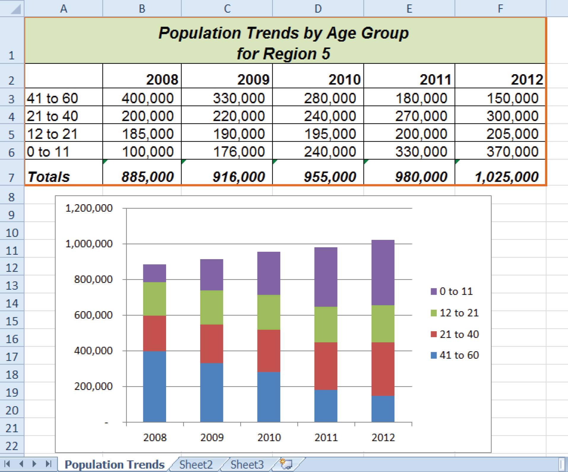
Integrity Check
Starter File: Chapter 1 IC Exercise 1
Difficulty: Level 3
The purpose of this exercise is to analyze a worksheet to determine whether there are any integrity flaws. First, read the scenario below. Then, open the file that is related to this exercise and analyze the worksheets contained in the workbook. You will find a worksheet in the workbook named AnswerSheet. This worksheet is to be used for any written responses required for this exercise.
Scenario
Your coworker provides you with sales data in an Excel workbook, which you intend to use for a sales strategy meeting with your boss. The workbook was attached to an e-mail with the following points stated in the message.
- The data represents the top-selling items for the company last year with respect to sales dollars.
- I received the data from an analyst in my department who insisted the cost data for each item was included. However, I don’t see it. You might have to manually enter this yourself. I included the cost for each item below.
- The original data I received is in Sheet1. I copied this data and pasted it into Sheet2. I thought you might like to see this sorted.
-
Cost per item data:
Item Cost Black Flat $35.00 Bracelet $30.00 Brown Pump $25.00 Daisy Print $40.00 Grey Stripe $110.00 Jersey Knit $80.00 Navy Pinstripe $125.00 Navy Wool $135.00 Quartz Watch $80.00 Sandal $45.00 Tan Trench $115.00 Topaz Ring $50.00
Assignment
- Analyze the data in this workbook carefully. Would you be comfortable using this data in a meeting with your boss? Use the AnswerSheet in this workbook to briefly list any concerns you have with this data.
- If it is necessary to enter the cost information, enter it in the Sheet1 worksheet. If not, state why in the AnswerSheet.
- Correct any problems and make any adjustments you think are appropriate to this workbook.
- Save the workbook by adding your name in front of the current workbook name.
Applying Excel Skills
The assignment in this section requires that you apply the skills presented in this chapter to achieve the stated objective. Read the assignment first and then open the file and complete the stated requirements. When you complete an assignment, save the file by adding your name in front of the current name of the workbook.
Starter File: Chapter 1 AES Assignment 1
Difficulty: Level 3
The workbook for this assignment contains sales plan data by month for merchandise categories sold by a hypothetical clothing retailer. Use the skills covered in this chapter to accomplish the points listed below.
- Show the total sales plan dollars next to each category in Column B.
-
Instead of showing the sales plan dollars by month, calculate the plan dollars for each quarter (see the following figure, “Layout for Sales by Quarter”). The months assigned to each quarter are as follows:
- Quarter 1: February, March, and April
- Quarter 2: May, June, and July
- Quarter 3: August, September, and October
- Quarter 4: November, December, and January
- Show the total plan for each quarter.
- Sort the merchandise categories based on the total sales plan dollars.
- Add any additional formatting enhancements that will make the worksheet easier to read.
Figure 1.68 Layout for Sales by Quarter
Chapter Skills Test
Starter File: Chapter 1 Skills Test
Difficulty: Level 2
Answer the following questions by executing the skills on the starter file required for this test. Answer each question in the order in which it appears. If you do not know the answer, skip to the next question. Open the starter file listed above before you begin this test.
- In the Sheet1 worksheet, enter the word Totals in cell C14.
- Format all the cells in Sheet1 to Arial font style and a 12-point font size.
- Set the character width for Columns A through G to 12.71.
- Edit the entry in cell B2 to read “Item Number.”
- Use AutoFill to fill the contents of cell B3 into the range B4:B13.
- Copy the contents of cell A3 and paste them into the range A4:A8.
- Delete Column F.
- Format the range A1:F2 so the text is Bold.
- Set the alignment in the range A2:F2 to Wrap Text.
- Change the fill color of the cells in the range A1:F1 to Red, Accent 2, Darker 25%.
- Make the following font changes to the range A1:F1: set the font color to white, add italics, and set the font size to 14.
- Merge and center the cells in the range A1:F1.
- Enter the title for this worksheet in the range A1:F1. The title should appear on two lines. The first line should read Status Report. The second line should read Sales and Inventory by Item.
- Increase the height of Row 1 so the entire title is visible.
- Insert a blank row above Row 14.
- Format the values in the range C3:C13 with a US dollar sign and two decimal places.
- Format the values in the range E3:F13 with zero decimal places and a comma at each thousands place.
- In cell E15, use AutoSum to calculate the sum of the values in the range E3:E14.
- Add vertical and horizontal lines to the range A1:F15.
- Add a bold line border around the perimeter of the range A1:F15.
- Insert a column chart using the data in the range D2:E13.
- Move the chart so the upper left corner is in the middle of cell H2.
- Sort the data in the range A2:F13 based on the values in the Sales in Units column. Sort the values in descending order or largest to smallest.
- Insert a new blank worksheet in the workbook.
- Delete Sheet3.
- Move Sheet4 ahead of Sheet2 so the order of the worksheets is Sheet1, Sheet4, and Sheet2.
- Rename the Sheet1 worksheet tab to “Status Report.”
- Change the orientation of the Status Report worksheet so it prints landscape instead of portrait.
- Adjust the appropriate settings so the Status Report worksheet prints on one piece of paper.
- Add a header to the Status Report worksheet that shows the date in the upper left corner and your name in the center.
- Add a footer to the Status Report worksheet that shows the page number in the lower right corner.
- Save the workbook by adding your name in front of the current workbook name (i.e., “your name Chapter 1 Skills Test”). (Hint: you will use Save As.)
- Close the workbook and Excel.