This is “Using Discounted Present Values”, section 4.2 from the book Theory and Applications of Microeconomics (v. 1.0). For details on it (including licensing), click here.
For more information on the source of this book, or why it is available for free, please see the project's home page. You can browse or download additional books there. To download a .zip file containing this book to use offline, simply click here.


4.2 Using Discounted Present Values
Learning Objectives
- When should you use the tool of discounted present value?
- How does an increase in the interest rate affect the discounted present value of a flow of income?
Section 4.1 "Consumption and Saving" introduced a valuable technique called discounted present value. You can use this technique whenever you need to compare flows of goods, services, or currencies (such as dollars) in different periods of time. In this section, we look at some of the big decisions you make during your life, both to illustrate discounted present value in action and to show how a good understanding of this idea can help you make better decisions.
Choosing a Career
A decision you typically make around the time that you graduate is your choice of a career. What makes the choice of a career so consequential is the fact that it can be very costly to switch from one career to another. For example, if you have trained as an engineer and then decide you want to be a lawyer, you will have to give up your engineering job (and give up your salary as well) and go to law school instead.
Suppose you are choosing among three careers: a lawyer, an insurance salesperson, or a barista. To make matters simple, we will work out an example with only two years. Table 4.2 "Which Career Should You Choose?" shows your earnings in each year at each occupation. In the first year in your career as a lawyer, we suppose that you work as a clerk, not earning very much. In the second year, you join a law firm and enjoy much higher pay. Selling insurance pays better than the legal career in the first year but worse in the second year. Working as a barista pays less than selling insurance in both years.
Table 4.2 Which Career Should You Choose?
| Career | First-Year Income ($) | Second-Year Income ($) |
|---|---|---|
| Lawyer | 5,000 | 60,000 |
| Insurance salesperson | 27,000 | 36,000 |
| Barista | 18,000 | 20,000 |
It is obvious that, if you care about the financial aspect of your career, you should not be a barista. (You would choose that career only if it had other benefits—such as flexible working hours and lack of stress—that outweighed the financial penalty.) It is less obvious whether it is better financially to work as a lawyer or as an insurance salesperson. Over the two years, you earn $65,000 as a lawyer and $63,000 as an insurance seller. But as we have already explained, simply adding your income for the two years is incorrect. The high salary you earn as a lawyer comes mostly in the second year and must be discounted back to the present.
To properly compare these careers, you should use the tool of discounted present value. With this tool, you can compare the income flows from the different occupations. Table 4.3 "Comparing Discounted Present Values of Different Income Streams" shows the discounted present value of the two-year flow of income for each career, assuming a 5 percent interest rate (that is, an interest factor equal to 1.05). Look, for example, at the lawyer’s income stream:
Similarly, the discounted present value of the income stream is $61,286 for the insurance salesperson and $37,048 for the barista. So if you are choosing your career on the basis of the discounted present value of your income stream, you should pick a career as a lawyer.
Table 4.3 Comparing Discounted Present Values of Different Income Streams
| Career | First-Year Income ($) | Second-Year Income ($) | Discounted Present Value at 5% Interest Rate ($) |
|---|---|---|---|
| Lawyer | 5,000 | 60,000 | 62,143 |
| Insurance salesperson | 27,000 | 36,000 | 61,286 |
| Barista | 18,000 | 20,000 | 37,048 |
This conclusion, however, depends on the interest rate used for discounting. Table 4.4 "Discounted Present Values with Different Interest Rates" adds another column, showing the discounted present values when the interest rate is 10 percent. You can see two things from this table: (1) The higher interest rate reduces the discounted present value for all three professions. If the interest rate increases, then future income is less valuable in present value terms. (2) The higher interest rate reverses our conclusion about which career is better. Selling insurance now looks better than being a lawyer because most of the lawyer’s earnings come in the future, so the discounting has a bigger effect.
Table 4.4 Discounted Present Values with Different Interest Rates
| Career | First-Year Income ($) | Second-Year Income($) | Discounted Present Value at 5% Interest Rate ($) | Discounted Present Value at 10% Interest Rate ($) |
|---|---|---|---|---|
| Lawyer | 5,000 | 60,000 | 62,143 | 59,545 |
| Insurance salesperson | 27,000 | 36,000 | 61,286 | 59,727 |
| Barista | 18,000 | 20,000 | 37,048 | 36,182 |
Of course, what you might really like to do is to sell insurance for the first year and work as a lawyer in the second year. This evidently would have higher income. Sadly, it is not possible: it is almost impossible to qualify for a high-paying lawyer’s job without investing a year as a law clerk first. Changing occupation can be very costly or even impossible if you don’t have the right skills. So choosing a career path means you must look ahead.
Going to College
If you are like most readers of this book, you have already made at least one very important decision in your life. You have chosen to go to college rather than taking a job immediately after graduating from high school. Ignoring the pleasures of going to college—and there are many—there are direct financial costs and benefits of a college education.
Think back to when you were deciding whether to go to college or to start work immediately. To keep our example from being too complicated, we again look at a two-year decision. What if you could obtain a college degree in one year, at a tuition cost of $13,000, and the interest rate is 5 percent annually? Your earnings are presented in Table 4.5 "Income from Going to College versus Taking a Job". In your year at college, you would earn no income, and you have to pay the tuition fee. In the following year, imagine that you can earn $62,143 working as a lawyer. Alternatively, you could bypass college and go to work as a barista, earning $10,000 in the first year and $37,048 in the second year. (We are assuming, as before, that you know these figures with certainty when you are making your decision.)
Table 4.5 Income from Going to College versus Taking a Job
| Career | Income in the Year at College ($) | Income in the Year after College ($) |
|---|---|---|
| College | −13,000 | 62,143 |
| Barista | 10,000 | 37,048 |
Going to college is an example of an investment decision. You incur a cost in the year when you go to college, and then you get a benefit in the future. There are two costs of going to college: (1) the $13,000 tuition you must pay (this is what you probably think of first when considering the cost of going to college) and (2) the opportunity cost of the income you could have earned while working. In our example, this is $10,000. The explicit cost and the opportunity cost together total $23,000, which is what it costs you to go to college instead of working in the first year.
By the way, we do not think about living expenses as a cost of going to college. You have to pay for food and accommodation whether you are at college or working. Of course, if these living expenses are different under the two scenarios, then you should take this into account. For example, if your prospective college is in New York City and has higher rental costs than in the city where you would work, then the difference in the rent should be counted as another cost of college.
The benefit of going to college is the higher future income that you enjoy. In our example, you will earn $62,143 in the following year if you go to college, and $37,048 if you do not. The difference between these is the benefit of going to college: $62,143 − $37,048 = $25,095. Even though this is greater than the $23,000 cost of going to college, we cannot yet conclude that going to college is a good idea. We have to calculate the discounted present value of this benefit. Suppose, as before, that the interest rate is 5 percent. Then
We can conclude that, with these numbers, going to college is a good investment. It is worth $900 more in discounted present value terms.
We could obtain this same conclusion another way. We could calculate the discounted value of the two-year income stream for the case of college versus barista, as in Table 4.6 "Income Streams from Going to College versus Taking a Job". We see that the discounted value of the income stream if you go to college is $46,184, compared to $45,284 if you work as a barista. The difference between these two is $900, just as before.
Table 4.6 Income Streams from Going to College versus Taking a Job
| Career | Income in the Year at College ($) | Income in the Year after College ($) | Discounted Present Value at 5% Interest Rate ($) |
|---|---|---|---|
| College | −13,000 | 62,143 | 46,184 |
| Barista | 10,000 | 37,048 | 45,284 |
You might have noticed that the figures we chose as “income in the year after college” in Table 4.5 "Income from Going to College versus Taking a Job" are the same as the numbers that we calculated in Table 4.3 "Comparing Discounted Present Values of Different Income Streams". The numbers in Table 4.3 "Comparing Discounted Present Values of Different Income Streams" were themselves the result of a discounted present value calculation: they were the discounted present value of a two-year income stream. When we compare going to college with being a barista, we are therefore calculating a discounted present value of something that is already a discounted present value. What is going on?
To understand this, suppose you are deciding about whether to go to college in 2012. If you do go to college, then in 2013 you will decide whether to be a lawyer, an insurance salesman, or a barista. If you decide on the legal career, then you will be a law clerk in 2013, and you will earn the high legal salary in 2014. Our analysis in Table 4.3 "Comparing Discounted Present Values of Different Income Streams" is therefore about the choice you make in 2013, thinking about your income in 2013 and 2014. Table 4.3 "Comparing Discounted Present Values of Different Income Streams" gives us the discounted present value in 2013 for each choice. If we then take those discounted present values and use them as “income in the year after college,” as in Table 4.6 "Income Streams from Going to College versus Taking a Job", we are in fact calculating the discounted present value, in 2012, of the flow of income you receive in 2012, 2013, and 2014.
If you think carefully about this, you will realize that
This is the same answer that we got before. As this example suggests, you can calculate discounted present values of long streams of income, including income you will receive many years in the future.The toolkit gives a more general formula for calculating the discounted present value. (See the more formal presentation of discounted present value at the end of Chapter 4 "Life Decisions", Section 4.4 "Embracing Risk".)
Economists have worked hard to measure the return on investment from schooling: “Alan B. Krueger, an economics professor at Princeton, says the evidence suggests that, up to a point, an additional year of schooling is likely to raise an individual’s earnings about 10 percent. For someone earning the national median household income of $42,000, an extra year of training could provide an additional $4,200 a year. Over the span of a career, that could easily add up to $30,000 or $40,000 of present value. If the year’s education costs less than that, there is a net gain.”Anna Bernasek, “What’s the Return on Education?” Economic View, Business Section, New York Times, December 11, 2005, accessed February 24, 2011, http://www.nytimes.com/2005/12/11/business/yourmoney/11view.html. Notice several things from this passage. First, the gains from education appear as an increase in earnings each year. So even if a 10 percent increase in earnings does not seem like a lot, it can be substantial once these gains are added over one’s lifetime. Second, Krueger is careful to use the term present value. Third, the number given is an average. Some people will benefit more; others will benefit less. Equally, some forms of schooling will generate larger income gains than others. Fourth, Krueger correctly notes that the present value must be compared with the cost of education, but you should remember that the cost of education includes the opportunity cost of lost income.
Table 4.7 "Return on Education" provides some more information on the financial benefits of schooling.US Census Bureau, “Income, Earnings, and Poverty from the American Community Survey,” 2010, table 5, accessed February 24, 2011, http://www.census.gov/hhes/www/poverty/publications/acs-01.pdf. The table shows average income in 2004. There is again evidence of a substantial benefit from schooling. Male college graduates, on average, earned more than $21,000 (68 percent) more than high school graduates, and female college graduates earned more than $16,000 (78 percent) more than high school graduates. The table shows that women are paid considerably less than men and also that the return on education is higher for women.
Table 4.7 Return on Education
| Schooling | Median Annual Income (Men) | Median Annual Income (Women) |
|---|---|---|
| High school graduate | 31,183 | 19,821 |
| Some college | 37,883 | 25,235 |
| College graduate | 52,242 | 35,185 |
Source: US Census Bureau, “Income, Earnings, and Poverty From the 2004 American Community Survey,” August 2005, table 5, page 10, accessed March 14, 2011, http://www.census.gov/hhes/www/poverty/publications/acs-01.pdf.
The presence of such apparently large gains from education helps explain why economists often suggest that education is one of the most important ingredients for the development of poorer countries. (In poorer countries, we are often talking not about the benefit of going to college but about the benefit of more years of high school education.) Moreover, the benefits from education typically go beyond the benefits to the individuals who go to school or college. There are benefits to society as a whole as well.
However, you should be careful when interpreting numbers such as these. We cannot conclude that if you randomly selected some high school graduates and sent them to college, then their income would increase by $17,000. As we all understand, individuals decide whether to go to college. These decisions reflect many things, including general intelligence, the ability to apply oneself to a task, and so on. People who have more of those abilities are more likely to attend—and complete—college.
One last point: we conducted this entire discussion “ignoring the pleasures of going to college.” But those pleasures belong in the calculations. Economics is about not only money but also all the things that make us happy. This is why we occasionally see people 60 years old or older in college. They attend not as an investment but simply because of the pleasure of learning. This is not inconsistent with economic reasoning or our discussion here. It is simply a reminder that your calculations should not only be financial but also include the all the nonmonetary things you care about.
The Effects of Interest Rates on Labor Supply
After you have decided whether or not to go to college and have chosen your career, you will still have plenty of decisions to make involving discounted present value. Remember that you have a lifetime budget constraint, in which the discounted present value of your income, including labor income, equals the discounted present value of consumption.
Your labor income is partly under your control. If you have some choice about how many hours to work, then your individual labor supply curve depends on the real wage, as shown in Figure 4.10 "Individual Labor Supply".Chapter 3 "Everyday Decisions" explains the individual supply of labor. The labor supply curve illustrates the fact that as the real wage increases, you are likely to work more. Labor supply, like the supply of loans that we considered previously, is driven by substitution and income effects. As the real wage increases,
- the opportunity cost of leisure increases, so you have an incentive to work more (substitution effect); and
- you have more income to spend on everything, including leisure, so you have an incentive to consume more leisure and work less (income effect).
Toolkit: Section 17.3 "The Labor Market"
The toolkit contains more information if you want to review the labor supply curve.
Figure 4.10 Individual Labor Supply
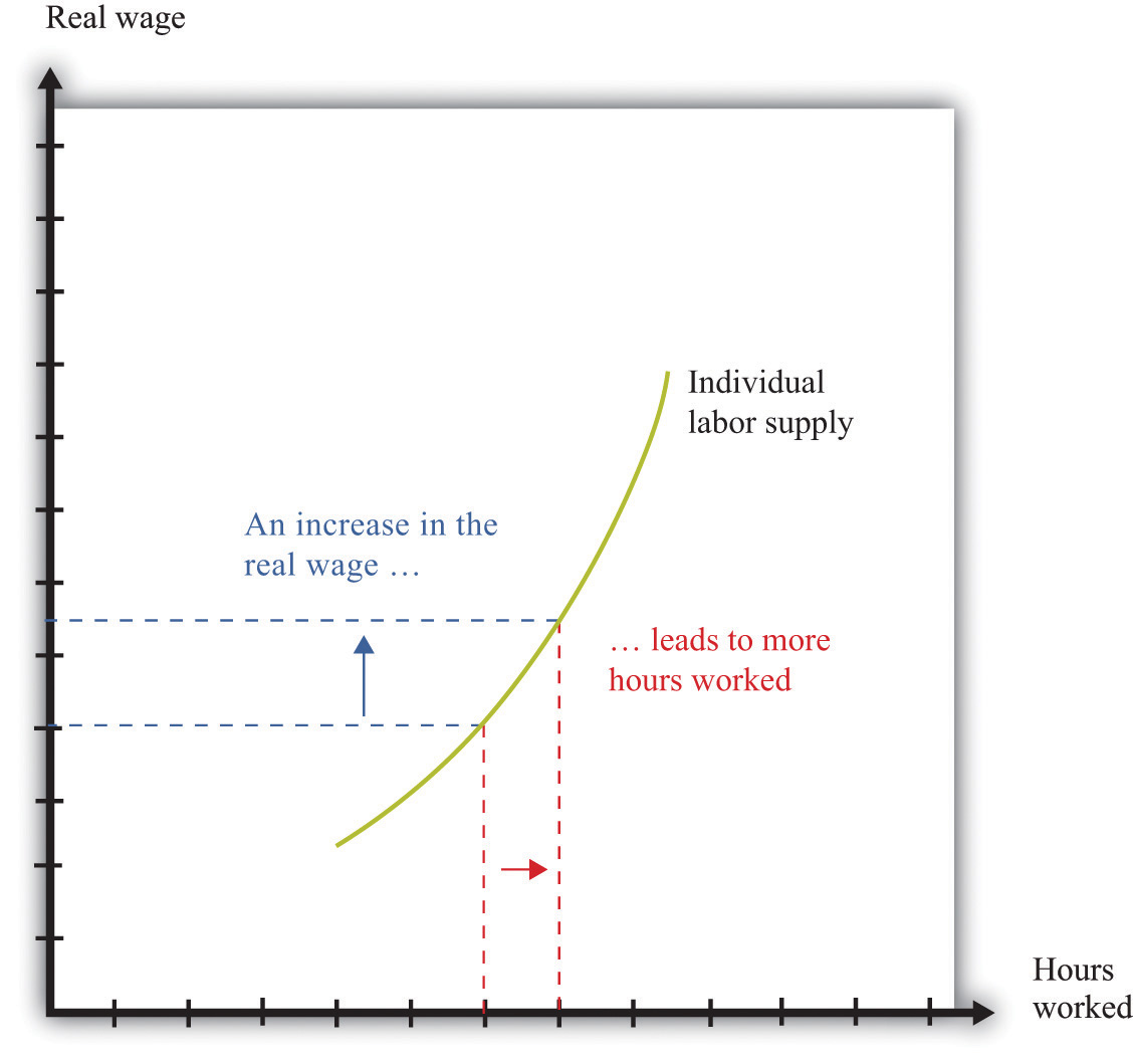
An increase in the real wage encourages an individual to work more. The labor supply curve slopes upward.
When you are making a decision about how much to work over many periods of time, your choice is more complicated. How much you choose to work right now depends not only on the real wage today but also on the real wage in the future and on the real interest rate. This is because you work both today and in the future to earn the income that goes into your lifetime budget constraint. If you think it is likely to be harder to earn money in the future, then you will probably decide to work more today. If you think it will be easier to earn money in the future, then you might well decide to work less today.
It is easiest to see how this works with an example. Suppose you are a freelance construction worker in Florida in the aftermath of a hurricane. There is lots of work available, and construction firms are paying higher than usual wages. You realize that you can earn much more per hour of work right now compared to your likely wage a few months in the future. A natural response is to work harder now to take advantage of the unusually high wages.
We can understand your decision in terms of income and substitution effects. The higher wage leads to the usual substitution effect. But because the change in the wage is only temporary, and because you are thinking about your wages over your lifetime, it does not have a large income effect. In this case, therefore, we expect the substitution effect to strongly outweigh the income effect.
Interest rates may also influence your decision about how hard to work. If interest rates increase, then the gains from working today increase as well. If you save money at high interest rates, you can enjoy more consumption in the future. High interest rates, like temporarily high current wages, increase the return to working today compared to working in the future, so you are likely to work more today.
The Demand for Durable Goods
Some of the products we purchase, such as milk or a ticket to a football game, disappear as soon as they are consumed. Other goods last for a long time and are, in effect, consumed over and over. Some examples are a bicycle, a car, and a microwave oven.
Goods that last over many uses are called durable goodsGoods that last over many uses., while those that do not last very long are called nondurable goodsGoods that do not last very long.. There is no hard-and-fast distinction between durable and nondurable goods. Many everyday items, such as plates, books, T-shirts, and downloaded music, are used multiple times. In economic statistics, however, the term durable is reserved for larger items that are bought only occasionally and that typically last for many years. Cars and kitchen appliances are classified as durable goods, but blue jeans and haircuts are not, even though they are not consumed all at once.
Because durable goods last a long time, making decisions about purchasing a durable good requires thinking about the future as well as the present. You must compare the benefits of the durable good over its entire lifetime relative to the cost you incur to pay for the durable now. A durable good purchase is typically a unit demand decision—you buy either a single unit or nothing. For unit demand, your decision rule is simple: buy if your valuation of the good exceeds the price of the good. (Remember that your valuation is the maximum you would be willing to pay for the good.) In the case of durable goods, there is an extra twist: your valuation needs to be a discounted present value.
Toolkit: Section 17.1 "Individual Demand"
You can review valuation and unit demand in the toolkit.
The idea is that you obtain a flow of services from a durable good. You need to place a valuation on that flow for the entire lifetime of the durable good. Then you need to calculate the discounted present value of that flow of services. If this discounted present value exceeds the price of the good, you should purchase it.
Suppose you are thinking of buying a new car that you expect to last for 10 years. You need to place a valuation on the flow of services that you get from the car each year: for example, you might decide that you are willing to pay $3,000 each year for the benefit of owning the car. To keep life really simple, let us think about a situation where the real interest rate is zero; this is the special case where it is legitimate to add these flows. So the car is worth $30,000 (= $3,000 per year × 10 years) to you now. This means you should be willing to buy the car if it costs less than $30,000, and you should not buy it otherwise.What if you think you might sell the car before it wears out? In this case, the value of the car has two components: (1) the flow of services you obtain while you own it, and (2) the price you can expect to obtain when you sell it. When you buy a durable good, you are purchasing an asset: something that yields some flow of benefits over time and that you can buy and sell. In general, the value of an asset depends on both the benefits that it provides and the price at which it can be traded. We examine these ideas in much more detail in Chapter 9 "Making and Losing Money on Wall Street".
If real interest rates are not zero, then spending on durable goods will depend on interest rates. As interest rates increase, the future benefits of the durable good become smaller, in terms of discounted present value. This means that durable goods become more expensive relative to nondurable goods. Thus the demand for durable goods decreases as interest rates increase.
One way to understand this is to realize that it is often easy to defer the purchase of a durable good. New durable goods are frequently bought to replace old goods that are wearing out. People buy new cars to replace their old cars or new washing machines to replace their old ones. If interest rates are high, you can often postpone such replacement purchases; you decide whether you can manage another year with your old car or leaking washing machine. As a result, spending on durable goods tends to be very sensitive to changes in interest rates.
These examples of discounted present value illustrate one key point: whenever you are making economics decisions about the future—be it what career to follow, when it is best to work hard, or if you should buy a new car—your decisions depend on the rate of interest. Whenever the rate of interest is high, future costs and benefits are substantially discounted and are therefore worth less in present value terms. High interest rates, in other words, mean that you put a lot of weight on the present relative to the future. When the rate of interest decreases, the future should play a larger role in your decisions.
Key Takeaways
- You should use discounted present value whenever you need to compare flows of income and expenses in different periods of time.
- The higher the interest rate, the lower the discounted present value of a flow.
Checking Your Understanding
- List five goods that are durable and five services that are nondurable. Is it possible to have a service that is durable?
- Calculate the appropriate values in Table 4.3 "Comparing Discounted Present Values of Different Income Streams" assuming an interest rate of 8 percent.
- If interest rates are lower, would you expect people to invest more or less in their health?