This is “Supply and Demand”, section 16.6 from the book Theory and Applications of Macroeconomics (v. 1.0). For details on it (including licensing), click here.
For more information on the source of this book, or why it is available for free, please see the project's home page. You can browse or download additional books there. To download a .zip file containing this book to use offline, simply click here.


16.6 Supply and Demand
The supply-and-demand framework is the most fundamental framework in economics. It explains both the price of a good or a service and the quantity produced and purchased.
The market supply curve comes from adding together the individual supply curves of firms in a particular market. A competitive firm, taking prices as given, will produce at a level such that
price = marginal cost.Marginal cost usually increases as a firm produces more output. Thus an increase in the price of a product creates an incentive for firms to produce more—that is, the supply curve of a firm is upward sloping. The market supply curve slopes upward as well: if the price increases, all firms in a market will produce more output, and some new firms may also enter the market.
A firm’s supply curve shifts if there are changes in input prices or the state of technology. The market supply curve is shifted by changes in input prices and changes in technology that affect a significant number of the firms in a market.
The market demand curve comes from adding together the individual demand curves of all households in a particular market. Households, taking the prices of all goods and services as given, distribute their income in a manner that makes them as well off as possible. This means that they choose a combination of goods and services preferred to any other combination of goods and services they can afford. They choose each good or service such that
price = marginal valuation.Marginal valuation usually decreases as a household consumes more of a product. If the price of a good or a service decreases, a household will substitute away from other goods and services and toward the product that has become cheaper—that is, the demand curve of a household is downward sloping. The market demand curve slopes downward as well: if the price decreases, all households will demand more.
The household demand curve shifts if there are changes in income, prices of other goods and services, or tastes. The market demand curve is shifted by changes in these factors that are common across a significant number of households.
A market equilibrium is a price and a quantity such that the quantity supplied equals the quantity demanded at the equilibrium price (Figure 16.4 "Market Equilibrium"). Because market supply is upward sloping and market demand is downward sloping, there is a unique equilibrium price. We say we have a competitive market if the following are true:
- The product being sold is homogeneous.
- There are many households, each taking the price as given.
- There are many firms, each taking the price as given.
A competitive market is typically characterized by an absence of barriers to entry, so new firms can readily enter the market if it is profitable, and existing firms can easily leave the market if it is not profitable.
Key Insights
- Market supply is upward sloping: as the price increases, all firms will supply more.
- Market demand is downward sloping: as the price increases, all households will demand less.
- A market equilibrium is a price and a quantity such that the quantity demanded equals the quantity supplied.
Figure 16.4 Market Equilibrium
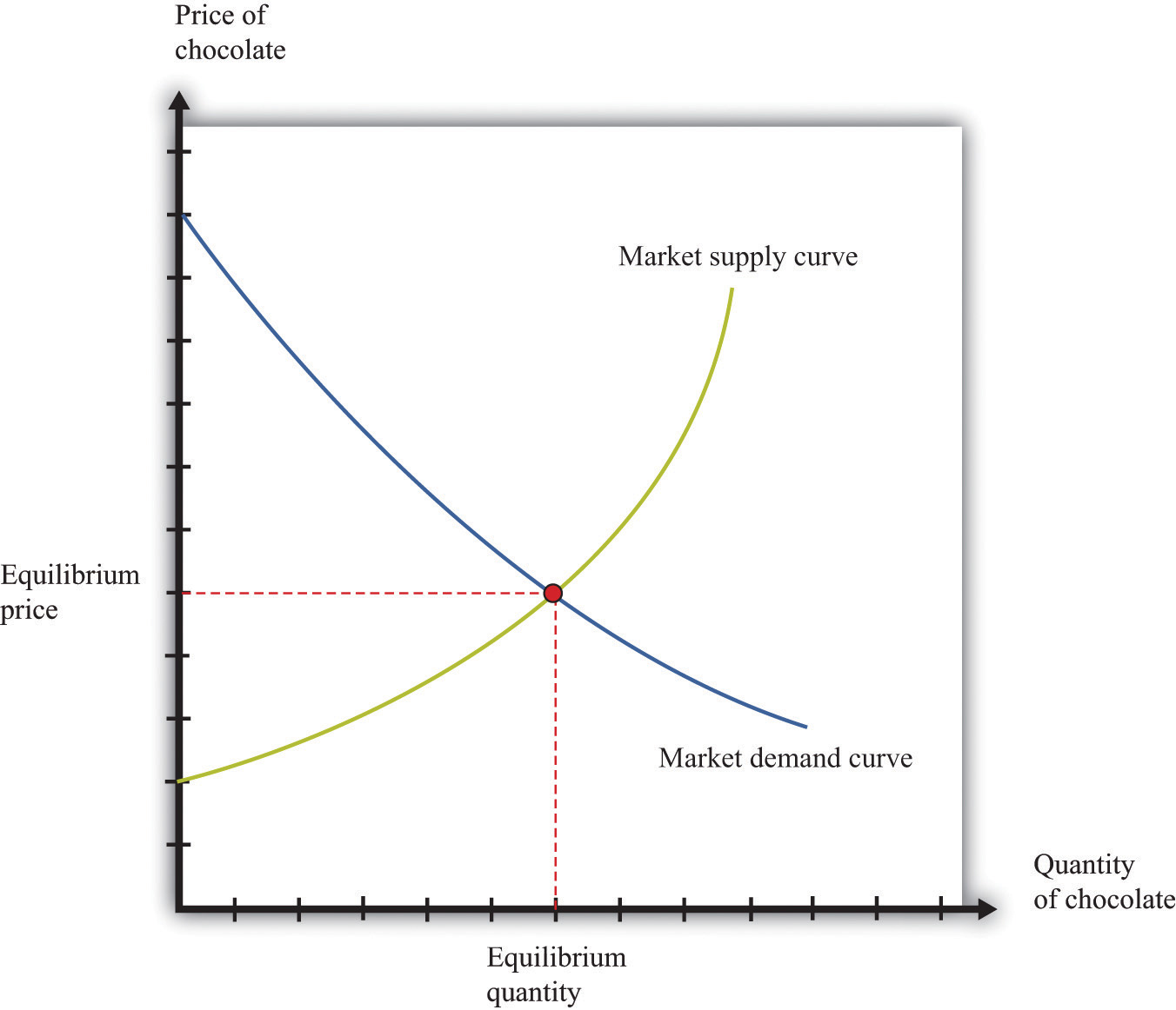
Figure 16.4 "Market Equilibrium" shows equilibrium in the market for chocolate bars. The equilibrium price is determined at the intersection of the market supply and market demand curves.
More Formally
If we let p denote the price, qd the quantity demanded, and I the level of income, then the market demand curve is given by
qd = a − bp + cI,where a, b, and c are constants. By the law of demand, b > 0. For a normal good, the quantity demanded increases with income: c > 0.
If we let qs denote the quantity supplied and t the level of technology, the market supply curve is given by
qs = d + ep + ft,where d, e, and f are constants. Because the supply curve slopes upward, e > 0. Because the quantity supplied increases when technology improves, f > 0.
In equilibrium, the quantity supplied equals the quantity demanded. Set qs = qd = q* and set p = p* in both equations. The market clearing price (p*) and quantity (q*) are as follows:
and
q* = d + ep* + ft.