This is “Inflations Big and Small”, chapter 26 from the book Theory and Applications of Economics (v. 1.0). For details on it (including licensing), click here.
For more information on the source of this book, or why it is available for free, please see the project's home page. You can browse or download additional books there. To download a .zip file containing this book to use offline, simply click here.


Chapter 26 Inflations Big and Small
Rising Prices
Through the years, people have been willing to wear some absurd slogans on their clothing. But surely one of the worst was the “WIN” button, introduced by United States President Gerald Ford in a speech on October 8, 1974.President Ford’s speech can be read and heard here: http://www.fordlibrarymuseum.gov/library/speeches/740121.asp. The button, shown in the following figure, was the symbol of a campaign against a perceived a social evil. And what was this great evil? It was inflation. “WIN” stood for “whip inflation now.” President Ford asked citizens to wear WIN buttons as a sign that they were enlisted in the battle against inflation.
Figure 26.1 Button: Whip Inflation Now

Wearing buttons might not have been the first bit of advice economists would have given to a leader interested in battling inflation. But this episode makes it evident that President Ford and his advisors viewed inflation as a major social problem. The president even invoked wartime imagery, concluding his speech by saying the following:President Ford’s speech can be read and heard here: http://www.fordlibrarymuseum.gov/library/speeches/740121.asp.
Only two of my predecessors have come in person to call upon Congress for a declaration of war, and I shall not do that. But I say to you with all sincerity that our inflation, our public enemy number one, will, unless whipped, destroy our country, our homes, our liberties, our property, and finally our national pride, as surely as any well-armed wartime enemy.
I concede there will be no sudden Pearl Harbor to shock us into unity and to sacrifice, but I think we have had enough early warnings. The time to intercept is right now. The time to intercept is almost gone.
My friends and former colleagues, will you enlist now? My friends and fellow Americans, will you enlist now? Together with discipline and determination, we will win.
When President Ford initiated this campaign, the US inflation rate was about 12 percent. In other words, a shirt that cost $10.00 in 1973 cost about $11.20 in 1974. This was the highest inflation rate that the United States had experienced since World War II. Inflation running at this rate is, at the very least, a significant inconvenience.
Still, compared to the experience of many countries, this level of inflation is negligible. Between World War I and World War II, Germany, Hungary, Austria, and Poland experienced massive rates of inflation. In one month in 1923, the annual inflation rate in Germany was 6,829 percent. This number is very difficult to fathom; it is astronomical compared to the inflation that President Ford was facing. At this rate of inflation, prices were doubling every three to four days.
Such rapid price increases forced people to change their behavior in extraordinary ways. The instant workers received their pay, they would rush out and spend it, for even a delay of a few hours could mean that your wages would buy fewer goods and services. Even ordering in a café became a game to beat inflation: “The price increases began to be dizzying. Menus in cafes could not be revised quickly enough. A student at Freiburg University ordered a cup of coffee at a cafe. The price on the menu was 5,000 Marks. He had two cups. When the bill came, it was for 14,000 Marks. ‘If you want to save money,” he was told, “and you want two cups of coffee, you should order them both at the same time.’”This comes from a PBS page with many excerpts about the German hyperinflation: “The German Hyperinflation, 1923,” Commanding Heights: The Battle for the World Economy, PBS, accessed September 20, 2011, http://www.pbs.org/wgbh/commandingheights/shared/minitext/ess_germanhyperinflation.html. And these are not just stories from long ago. In the past 25 years, there have been large inflations in Yugoslavia, Israel, Argentina, Brazil, Mexico, Ukraine, and Zimbabwe, for example.
What is the cause of inflation?
Road Map
In this chapter, we study the causes and consequences of inflation. Times of rapid inflation are especially helpful for understanding inflation in general. When inflation is the dominant feature of an economy, it is very easy to isolate the main forces at work. We will see, moreover, that the most interesting periods to study are the beginning and end of large inflations, for such times provide a particular insight into the connection between fiscal policy and monetary policy.
We first study the relationship between the inflation rate and changes in the amount of money circulating in an economy and explain that, in the long run, there is a close connection between the inflation rate and the growth rate of the money supply. We look at some data both for the United States and for other countries and examine some examples of hyperinflation. Then we explore the underlying cause of hyperinflations, which turn out to be connected to the tax and spending choices that governments make, and we conclude by discussing government policy to control inflation.
26.1 The Quantity Theory of Money
Learning Objectives
After you have read this section, you should be able to answer the following questions.
- What is the quantity theory of money?
- What is the classical dichotomy?
- According to the quantity theory, what determines the inflation rate in the long run?
We begin by presenting a framework to highlight the link between money growth and inflation over long periods of time.The framework complements our discussion of inflation in the short run, contained in Chapter 25 "Understanding the Fed". The quantity theory of moneyA relationship among money, output, and prices that is used to study inflation. is a relationship among money, output, and prices that is used to study inflation. It is based on an accounting identity that can be traced back to the circular flow of income. Among other things, the circular flow tells us that
nominal spending = nominal gross domestic product (GDP).The “nominal spending” in this expression is carried out using money. While money consists of many different assets, you can—as a metaphor—think of money as consisting entirely of dollar bills. Nominal spending in the economy would then take the form of these dollar bills going from person to person. If there are not very many dollar bills relative to total nominal spending, then each bill must be involved in a large number of transactions.
The velocity of moneyNominal GDP divided by the money supply. is a measure of how rapidly (on average) these dollar bills change hands in the economy. It is calculated by dividing nominal spending by the money supply, which is the total stock of money in the economy:
If the velocity is high, then for each dollar, the economy produces a large amount of nominal GDP.
Using the fact that nominal GDP equals real GDP × the price level, we see that
And if we multiply both sides of this equation by the money supply, we get the quantity equationAn equation stating that the supply of money times the velocity of money equals nominal GDP., which is one of the most famous expressions in economics:
money supply × velocity of money = price level × real GDP.Let us see how these equations work by looking at 2005. In that year, nominal GDP was about $13 trillion in the United States. The amount of money circulating in the economy was about $6.5 trillion.In Chapter 24 "Money: A User’s Guide", we discussed the fact that there is no simple single definition of money. This figure refers to a number called “M2,” which includes currency and also deposits in banks that are readily accessible for spending. If this money took the form of 6.5 trillion dollar bills changing hands for each transaction that we count in GDP, then, on average, each bill must have changed hands twice during the year (13/6.5 = 2). So the velocity of money was 2 in 2005.
Toolkit: Section 31.27 "The Circular Flow of Income"
You can review the circular flow of income in the toolkit.
The Classical Dichotomy
So far, we have just written a definition. There are two steps that take us from this definition to a theory of inflation. First we use the quantity equation to give us a theory of the price level. Then we examine the growth rate of the price level, which is the inflation rate.
In macroeconomics we are always careful to distinguish between nominal and real variables:
- Nominal variablesA variable defined and measured in terms of money. are defined and measured in terms of money. Examples include nominal GDP, the nominal wage, the dollar price of a carton of milk, the price level, and so forth. (Most nominal variables are measured in monetary units, but some are just numbers. For example, the nominal interest rate tells you how many dollars you will obtain next year for each dollar you invest in an asset this year. It is thus measured as “dollars per dollar,” so it is a number.)
- All variables not defined or measured in terms of money are real variablesA variable defined and measured in terms other than money, often in terms of real GDP.. They include all the variables that we divide by a price index in order to correct for the effects of inflation, such as real GDP, real consumption, the capital stock, the real wage, and so forth. For the sake of intuition, you can think of these variables as being measured in terms of units of (base year) GDP (so when we talk about real consumption, for example, you can think about the actual consumption of a bundle of goods and services by a household). Real variables also include the supply of labor (measured in hours) and many variables that have no specific units but are just numbers, such as the velocity of money or the capital-to-output ratio of an economy.
Prior to the Great Depression, the dominant view in economics was an economic theory called the classical dichotomyThe dichotomy that real variables are determined independently of nominal variables.. Although this term sounds imposing, the idea is not. According to the classical dichotomy, real variables are determined independently of nominal variables. In other words, if you take the long list of variables used by macroeconomists and write them in two columns—real variables on the left and nominal variables on the right—then you can figure out all the real variables without needing to know any of the nominal variables.
Following the Great Depression, economists turned instead to the aggregate expenditure modelThe relationship between planned spending and output. to better understand the fluctuations of the aggregate economy. In that framework, the classical dichotomy does not hold. Economists still believe the classical dichotomy is important, but today economists think that the classical dichotomy only applies in the long run.
The classical dichotomy can be seen from the following thought experiment. Start with a situation in which the economy is in equilibrium, meaning that supply and demand are in balance in all the different markets in the economy. The classical dichotomy tells us that this equilibrium determines relative prices (the price of one good in terms of another), not absolute prices. We can understand this result by thinking about the markets for labor, goods, and credit.
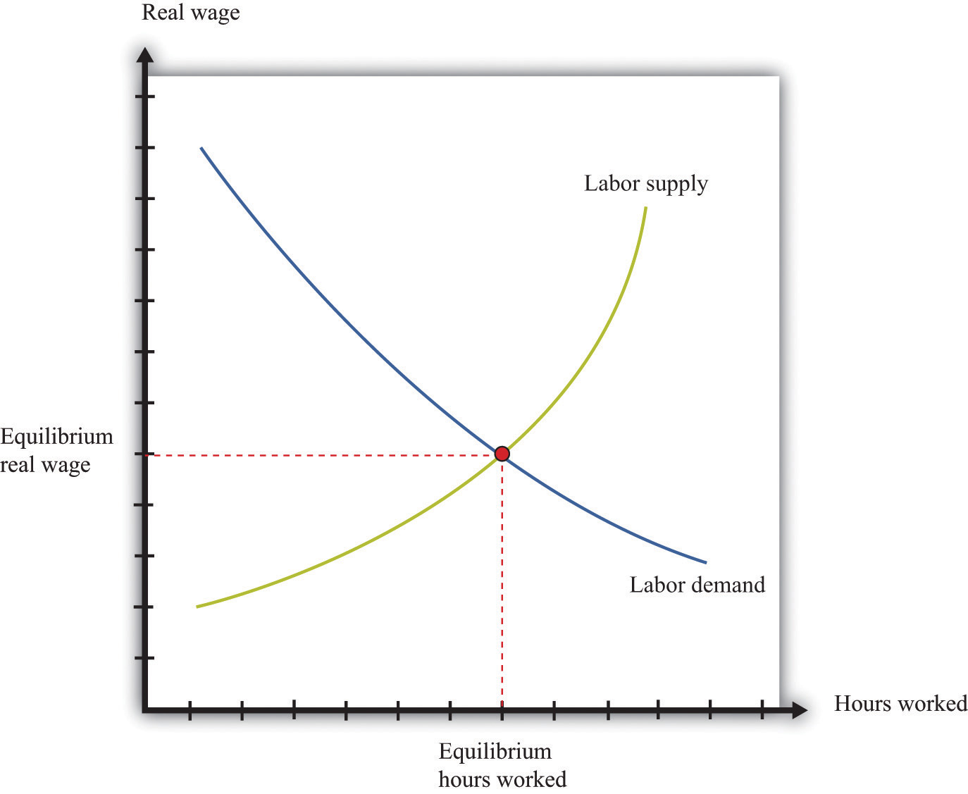
Figure 26.2 "Labor Market Equilibrium" presents the labor market equilibrium. On the vertical axis is the real wage because households and firms make their labor supply and demand decisions based on real, not nominal, wages. Households want to know how much additional consumption they can get by working more, whereas firms want to know the cost of hiring more labor in terms of output. In both cases, it is the real wage that determines economic choices.
Figure 26.2 Labor Market Equilibrium
Now think about the markets for goods and services. The demand for any good or service depends on the real income of households and the real price of the good or service. We can calculate real prices by correcting for inflation: that is, by dividing each nominal price by the aggregate price level. Household demand decisions depend on real variables, such as real income and relative prices.If you have studied the principles of microeconomics, remember that the budget constraint of a household depends on income divided by the price of one good and on the price of one good in terms of another. If there are multiple goods, the budget constraint can be determined by dividing income by the price level and by dividing all prices by the same price level. The same is true for the supply decisions of firms. We have already argued that labor demand depends on only the real wage. Hence the supply of output also depends on the real, not the nominal, wage. More generally, if the firm uses other inputs in the production process, what matters to the firm’s decision is the price of these inputs relative to the price of its output, or—more generally—relative to the overall price level.If you have studied the principles of microeconomics, the condition that price equals marginal cost is used to characterize the output decision of a firm. What matters then is the price of the input, relative to the price of output.
What about credit markets? The supply and demand for credit depends on the real interest rate. This means that those supplying credit think about the return they receive on making loans in real terms: although the loan may be stated in terms of money, the supply of credit actually depends on the real return. The same is true for borrowers: a loan contract may stipulate a nominal interest rate, but the real interest rate determines the cost of borrowing in terms of goods. The supply of and demand for credit is illustrated in Figure 26.3 "Credit Market Equilibrium".
Figure 26.3 Credit Market Equilibrium
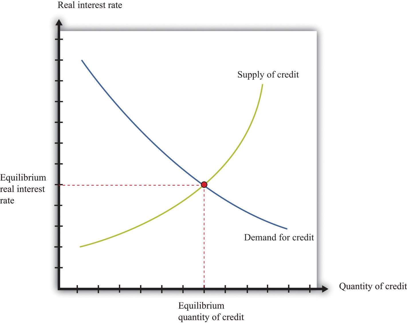
The credit market equilibrium occurs at a quantity of credit extended (loans) and a real interest rate where the quantity supplied is equal to the quantity demanded.
Toolkit: Section 31.3 "The Labor Market", Section 31.24 "The Credit (Loan) Market (Macro)", and Section 31.8 "Correcting for Inflation"
You can review the labor market and the credit market, together with the underlying demand and supply curves, in the toolkit. You can also review how to correct for inflation.
The classical dichotomy has a key implication that we can study through a comparative statics exercise. Recall that in a comparative statics exercise we examine how the equilibrium prices and output change when something else, outside of the market, changes. Here we ask: what happens to real GDP and the long-run price level when the money supply changes? To find the answer, we begin with the quantity equation:
money supply × velocity of money = price level × real GDP.Previously we discussed this equation as an identity—something that must be true by the definition of the variables. Now we turn it into a theory. To do so, we make the assumption that the velocity of money is fixed. This means that any increase in the money supply must increase the left-hand side of the quantity equation. When the left-hand side of the quantity equation increases, then, for any given level of output, the price level is higher (equivalently, for any given value of the price level, the level of real GDP is higher).
What then changes when we change the money supply: output, prices, or both? Based on the classical dichotomy, we know the answer. Real variables, such as real GDP and the velocity of money, stay constant. A change in a nominal variable—the money supply—leads to changes in other nominal variables, but real variables do not change. The fact that changes in the money supply have no long-run effect on real variables is called the long-run neutrality of moneyThe fact that changes in the money supply have no long-run effect on real variables..
Toolkit: Section 31.16 "Comparative Statics"
You can find more details on how to conduct comparative static exercises in the toolkit.
How does this view of the effects of monetary policy fit with the monetary transmission mechanismA mechanism explaining how the actions of a central bank affect aggregate economic variables, in particular real GDP.?See Chapter 25 "Understanding the Fed". The monetary transmission mechanism explains that the monetary authority affects aggregate spending by changing its target interest rate.
- The monetary authority changes interest rates.
- Changes in interest rates influence spending on durables by firms and households.
- Changes in spending influence aggregate spending through a multiplier effect.
Remember that the monetary authority changes interest rates through open-market operations. If it wants to boost aggregate spending, it does so by cutting interest rates, and it cuts interest rates by purchasing government bonds with money. An interest rate cut is equivalent to an increase in the supply of money, so the monetary transmission mechanism also teaches us that an increase in the supply of money leads to an increase in aggregate spending.There is one difference, unimportant here, which is that the monetary transmission mechanism does not necessarily suppose that the velocity of money is constant. The monetary transmission mechanism is useful when we want to understand the short-run effects of monetary policy. When studying the long run, it is easier to work with the quantity equation and to think about monetary policy in terms of the supply of money rather than interest rates.
Finally, a reminder: in the short run, the neutrality of money does not hold. This is because in the short run we assume stickiness of nominal wages and/or prices. In this case, changes in the nominal money supply will lead to changes in the real money supply. With sticky wages and/or prices, the classical dichotomy is broken.
Long-Run Inflation
We now use the quantity equation to provide us with a theory of long-run inflation. To do so, we use the rules of growth rates. One of these rules is as follows: if you have two variables, x and y, then the growth rate of the product (x × y) is the sum of the growth rate of x and the growth rate of y. We can apply this to the quantity equation:
money supply × velocity of money = price level × real GDP.The left side of this equation is the product of two variables, the money supply and the velocity of money. The right side is likewise the product of two variables. So we obtain
growth rate of the money supply + growth rate of the velocity of money = inflation rate + growth rate of output.We have used the fact that the growth rate of the price level is, by definition, the inflation rate.
Toolkit: Section 31.21 "Growth Rates"
You can review the rules of growth rates in the toolkit.
We continue to assume that the velocity of money is a constant.In fact, the velocity of money might also grow over time as a result of developments in the financial sector. Saying that the velocity of money is constant is the same as saying that its growth rate is zero. Using this fact and rearranging the equation, we discover that the long-run inflation rate depends on the difference between how rapidly the money supply grows and how rapidly output grows:
inflation rate = growth rate of money supply − growth rate of output.The long-run growth rate of output does not depend on the growth rate of the money supply or the inflation rate. We know this because long-run output growth depends on the accumulation of capital, labor, and technology. From our discussion of labor and credit markets, equilibrium in these markets is described by real variables. Equilibrium in the labor market depends on the real wage and not on any nominal variables. Likewise, equilibrium in the credit market tells us that the level of investment does not depend on nominal variables. Since the capital stock in any period is just the accumulation of past investment, we know that the stock of capital is also independent of nominal variables.
Therefore there is a direct link between the money supply growth rate and the inflation rate. The classical dichotomy teaches us that changes in the money supply do not affect the velocity of money or the level of output. It follows that any changes in the growth rate of the money supply will show up one-for-one as changes in the inflation rate. We say more about monetary policy later, but notice that there are immediate implications for the conduct of monetary policy:
- In a growing economy, there are more transactions taking place, so there is typically a need for more money to facilitate those transactions. Thus some growth of the money supply is probably desirable to match the increased income.
- If the monetary authorities want a stable price level—zero inflation—in the long run, then they should try to set the growth rate of the money supply equal to the (long-run) growth rate of output.
- If the monetary authorities want a low level of inflation in the long run, then they should aim to have the money supply grow just a little bit faster than the growth rate of output.
Keep in mind that this is just a theory. The quantity equation holds as an identity. But the assumption of constant velocity and the statement that long-run output growth is independent of money growth are assertions based on a body of theory. We now look at how well this theory fits the facts.
Key Takeaways
- The quantity theory of money states that the supply of money times the velocity of money equals nominal GDP.
- According to the classical dichotomy, real variables, such as real GDP, consumption, investment, the real wage, and the real interest rate, are determined independently of nominal variables, such as the money supply.
- Using the quantity equation along with the classical dichotomy, in the long run the inflation rate equals the rate of money growth minus the growth rate of output.
Checking Your Understanding
- Is the real wage a nominal variable? What about the money supply?
- If velocity of money decreases by 2 percent and the money supply does not grow, can you say what will happen to nominal GDP growth? Can you say what will happen to inflation?
26.2 Facts about Inflation and Money Growth
Learning Objectives
After you have read this section, you should be able to answer the following questions:
- What does it mean to say that “inflation is always and everywhere a monetary phenomenon”?
- What do we know about inflation and money growth in the United States?
- What happened during past and recent hyperinflations?
According to the quantity equation, the inflation rate and the rate of money growth are closely linked. As the famous economist Milton Friedman said, “Inflation is always and everywhere a monetary phenomenon.”This quote comes from Milton Friedman and Anna Schwartz, A Monetary History of the United States, 1867–1960 (Princeton, NJ: Princeton University Press, 1963). By this he meant that inflation could always ultimately be traced to “excessive” money growth. Keep in mind that we are talking about the long run here. Over shorter periods of time, changes in the money supply affect the level of real economic activity and have correspondingly less effect on the inflation rate.
Inflation and Money Growth in the United States
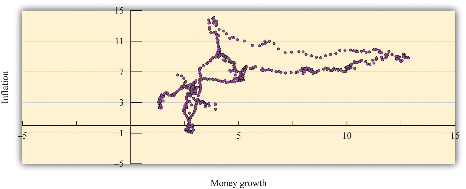
Figure 26.4 "Inflation and Money Growth in the Short Run" and Figure 26.5 "Inflation and Money Growth in the Long Run" show the relationship between inflation and money growth for the United States. For this discussion, money growth is measured as M1. The rate of money growth is on the horizontal axis, and the annual inflation rate is on the vertical axis.
Figure 26.4 Inflation and Money Growth in the Short Run
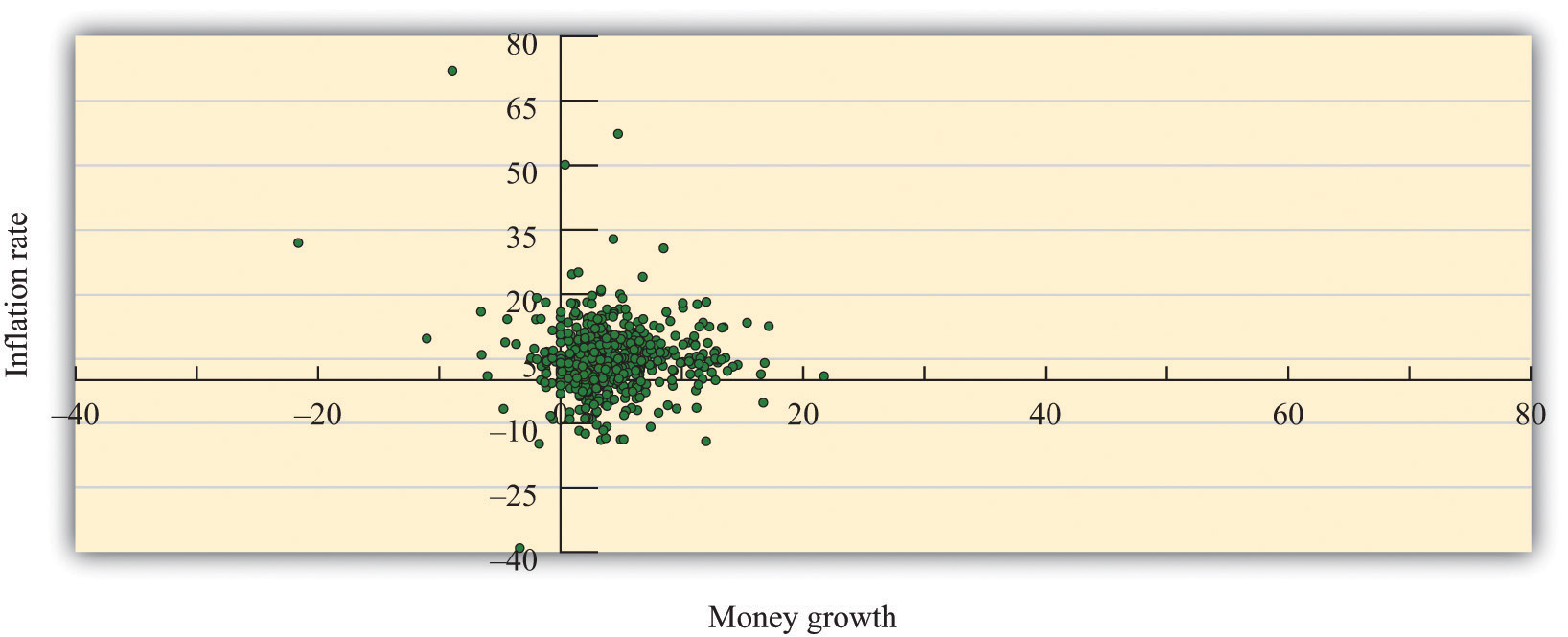
Figure 26.5 Inflation and Money Growth in the Long Run
The two figures differ in the time horizon used to compute the growth rates. In Figure 26.4 "Inflation and Money Growth in the Short Run", month-to-month changes in money and prices are used to calculate annual growth rates. If you listen to a radio report or read the newspaper about inflation, typically you will first be told about the monthly Consumer Price Index (CPI) and then be given an annual inflation rate. The annual growth rate is the amount by which the variable would increase if the monthly growth rate persisted for a year. The conversion is simply to take the monthly percentage change and convert it into an annual percentage change by multiplying by 12. So if the CPI increased from 112 to 118 over the past month, then the change for the month would be calculated as follows:
If prices increased at this rate each month at this same rate, then prices would increase by 12 × 5.36 percent = 64.32 percent over the year. The data for Figure 26.4 "Inflation and Money Growth in the Short Run" start in January 1959 and end in December 2010. So the first observation is the annual percentage change between January and February 1959.
Figure 26.5 "Inflation and Money Growth in the Long Run" examines annual growth rates based on observing the money supply and the price level at five-year intervals. The first observation is the annual growth rate for the period starting in January 1959 and ending in January 1964. The annual growth rates for a five-year period are computed for each month starting in January 1964. Here, instead of multiplying a monthly growth rate by 12 to get an annual rate, we divide a five-year rate by 5 to get an annual rate. The point of examining growth rates over longer periods of time goes back to the idea that we are investigating the relationship between prices and the money supply over long periods of time.
Comparing these two figures, you can see that the relationship between money growth and inflation is much tighter when we examine five-year periods, as in Figure 26.5 "Inflation and Money Growth in the Long Run", rather than the monthly changes in Figure 26.4 "Inflation and Money Growth in the Short Run". This is consistent with the view that the relationship between money growth and inflation is a long-term relationship, not a short-term relationship.
In the monthly data, the link between money growth and inflation is relatively weak. The correlation, a measure of how closely two variables move together, is only 0.20 in the monthly data. In contrast, for the annual growth rates computed by looking over a five-year period, the correlation is about 0.65, indicating that money growth and inflation move more closely together over longer periods of time.
Toolkit: Section 31.23 "Correlation and Causality"
You can review the meaning and measurement of correlation in the toolkit.
Money Growth and Inflation in Other Countries
In the United States, money growth and inflation rates are relatively moderate. Looking back at Figure 26.5 "Inflation and Money Growth in the Long Run", we see that the highest inflation rate in the past half-century was about 15 percent, in 1980. Some other countries have had a very different experience.
Figure 26.6 "Inflation and Money Growth in Different Countries" shows data on money growth and inflation from 110 countries.See George McCandless Jr. and Warren Weber, “Some Monetary Facts,” Federal Reserve Bank of Minneapolis Quarterly Review 19, no. 3 (Summer 1995): 2–11. The article provides a complete description of the data and the countries. On the vertical axis of the figure is the inflation rate, measured as the annual rate of change of the CPI. On the horizontal axis is the rate of growth of the money supply. So a point in the figure represents a single country and shows that country’s combination of inflation and money growth. The sample period used is 1960–1990, meaning that each point is an average over a three-decade period.
Figure 26.6 Inflation and Money Growth in Different Countries
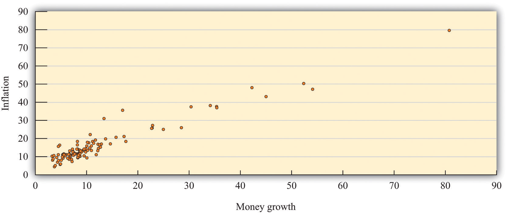
Figure 26.6 "Inflation and Money Growth in Different Countries" clearly indicates that countries with high money growth are the countries that experience high inflation. If you were to draw a line through the points that came as close as possible to them, that line would have a positive slope. McCandless and Weber conclude as follows: “In the long run, there is a high (almost unity) correlation between the rate of growth of the money supply and the inflation rate. This holds across three definitions of money and across the full sample of countries and two subsamples.”George McCandless Jr. and Warren Weber, “Some Monetary Facts,” Federal Reserve Bank of Minneapolis Quarterly Review 19, no. 3 (Summer 1995): 2–11.
Big Inflations
Most of the countries in Figure 26.6 "Inflation and Money Growth in Different Countries" have inflation and money growth that are less than 20 percent. There are some outliers, however. For example, there is one country with inflation and money growth at 80 percent annually over the sample. This country is Argentina; we return to it later. There have been episodes in history where the rates of inflation were so large that they are difficult to comprehend.
Germany, 1922–24
Table 26.1 "Prices in Germany" contains data for Germany in the early 1920s.The data come from Thomas Sargent, “The Ends of Four Big Inflations,” in Inflation: Causes and Effects, ed. Robert Hall (Cambridge, MA: National Bureau of Economic Research, 1982). The data in this case show the levels of wholesale prices because reliable consumer price indices were not available. The second column is a measure of prices for each month, from January 1922 to June 1924. The third column computes the annual inflation rate by multiplying the monthly inflation rate by 12. The final column indicates the amount of time in days it would take for prices to double at the annual inflation rate indicated in the third column. (When the number in the last column is negative, it tells you how long it would take the price level to halve.)
Table 26.1 Prices in Germany
| Month and Year | Price Level | Annual Growth Rate (%) | Doubling Time in Days |
|---|---|---|---|
| January 1922 | 3,670 | 60.3 | 419 |
| February 1922 | 4,100 | 133.0 | 190 |
| March 1922 | 5,430 | 337.1 | 75 |
| April 1922 | 6,360 | 189.7 | 133 |
| May 1922 | 6,460 | 18.7 | 1351 |
| June 1922 | 7,030 | 101.5 | 249 |
| July 1922 | 10,160 | 441.9 | 57 |
| August 1922 | 19,200 | 763.7 | 33 |
| September 1922 | 28,700 | 482.4 | 52 |
| October 1922 | 56,600 | 814.9 | 31 |
| November 1922 | 115,100 | 851.8 | 30 |
| December 1922 | 147,480 | 297.5 | 85 |
| January 1923 | 278,500 | 762.9 | 33 |
| February 1923 | 588,500 | 897.8 | 28 |
| March 1923 | 488,800 | −222.7 | −113.6 |
| April 1923 | 521,200 | 77.0 | 328 |
| May 1923 | 817,000 | 539.4 | 47 |
| June 1923 | 1,938,500 | 1036.8 | 24 |
| July 1923 | 7,478,700 | 1620.2 | 16 |
| August 1923 | 94,404,100 | 3042.6 | 8 |
| September 1923 | 2,394,889,300 | 3880.2 | 6 |
| October 1923 | 709,480,000,000 | 6829.4 | 4 |
| November 1923 | 72,570,000,000,000 | 5553.3 | 5 |
| December 1923 | 126,160,000,000,000 | 663.6 | 38 |
| January 1924 | 117,320,000,000,000 | −87.2 | −290 |
| February 1924 | 116,170,000,000,000 | −11.8 | −2140 |
| March 1924 | 120,670,000,000,000 | 45.6 | 555 |
| April 1924 | 124,050,000,000,000 | 33.2 | 763 |
| May 1924 | 122,460,000,000,000 | −15.5 | −1634 |
| June 1924 | 115,900,000,000,000 | −66.1 | −383 |
From the table, you can get a vivid sense of the pace of prices simply by counting the number of digits used to describe the price level. At the height of the inflation in October 1923, the annual inflation rate was over 6,800 percent. It is hard to make sense of a number like this, which is why we include the fourth column: at this inflation rate, prices double every 3 to 4 days. Rapid inflation of this kind is called hyperinflationA period of very high and often escalating inflation..
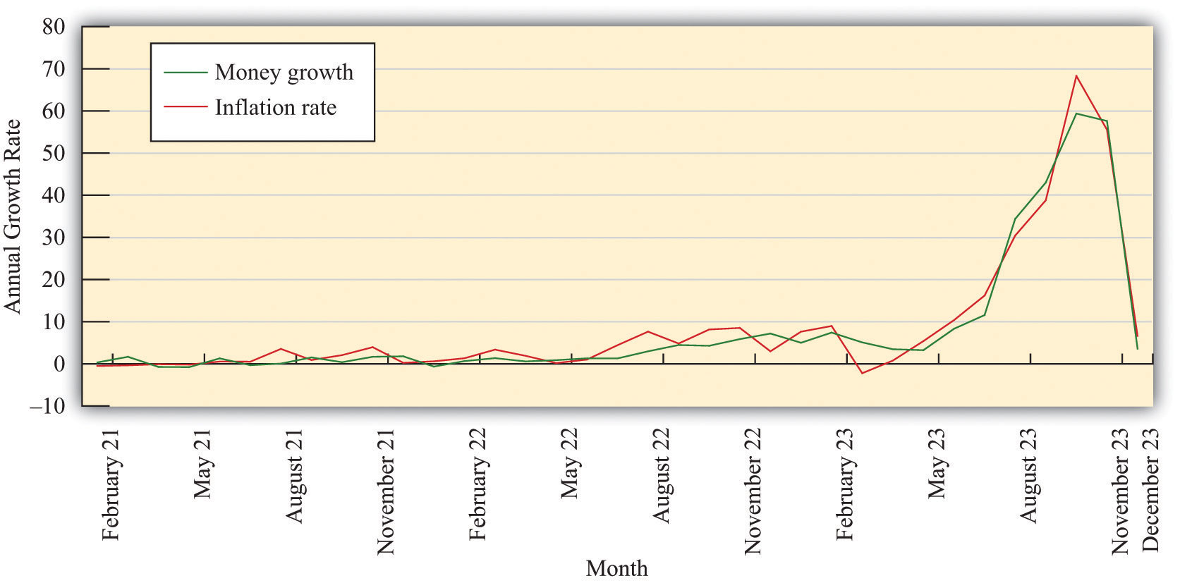
Where does hyperinflation come from? The quantity theory tells us that the rapid price increases must be related to growth in the money supply, a reduction in output growth, or rapid growth in the velocity of money. Drawing on the quote from Milton Friedman, it is natural to first examine the growth rate of the money supply. Figure 26.7 "Money Growth and Inflation in Germany" shows the money growth and inflation rates for Germany during this period. The graph clearly shows that as prices were exploding in Germany, so too was the money supply. In 1922, prices increased 93 percent, and the money stock grew at 52 percent. In the following year, the average inflation rate was up to 433 percent, and the money supply grew at almost 300 percent.These are calculated as January to January growth rates.
In October 1923, when the inflation rate peaked at over 6,800 percent, the money supply grew at nearly 6,000 percent on an annual basis. According to economist Thomas Sargent, 99 percent of the outstanding bank notes had been put in circulation during the previous month. At that point, both prices and the money supply were doubling in a matter of days. Thus the escalating prices were matched by enormous increases in the money supply.
Figure 26.7 Money Growth and Inflation in Germany
At first glance, the German data seem to confirm the idea that large inflation rates are driven by large money growth rates. On closer examination, though, we notice that the inflation rates were greater than the growth rate of the money supply. Yet we said earlier that
inflation rate = growth rate of money supply + growth rate of velocity − growth rate of output.It follows that the velocity of money must have been increasing or output must have been decreasing.
It is plausible, indeed likely, that the velocity of money will increase during a period of very high inflation. If you know that the cash in your pocket will lose its value from one hour to the next, then you want to get rid of it quickly. During the German hyperinflation, anyone with cash wanted to exchange it as quickly as possible for goods and services. Thus money changed hands more and more rapidly: in other words, the velocity of money increased.
Money had ceased to perform one of its key functions. It was no longer a store of value. Even if people were still using money as a medium of exchange, they could no longer rely on money to keep its value. A monetary system is a fragile institution: its success depends on everyone believing in it.See Chapter 24 "Money: A User’s Guide" for more discussion. People are willing to accept money because they think that others will, in turn, be willing to accept it from them. During a hyperinflation, this system breaks down. People are reluctant to accept money because they know that others will not want to accept it from them.
Rapid inflation is also disruptive to the general functioning of the economy. People have to devote much more time and energy to managing their cash. People insist on being paid more frequently and abandon work to shop as soon as they are paid. Furthermore, as discussed later, inflation acts as a tax on work. So higher inflation means a higher tax and thus a reduction in employment and output. Overall, output does tend to decrease during hyperinflation, increasing the inflation rate still further. For Germany, real output decreased by 46 percent in 1923 during the height of the hyperinflation. In contrast, 1924 was a good year for the economy, with real output growing at 35 percent.
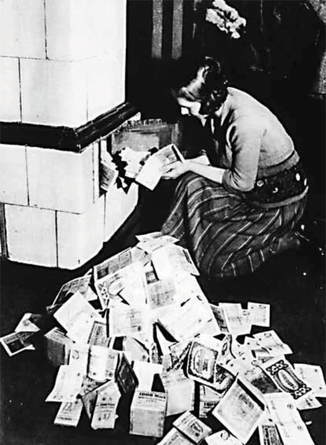
So while rapid money growth sets hyperinflation in motion, hyperinflation then becomes self-fueling, powered by increases in the velocity of money and—to a minor extent—decreases in the growth rate of output. In the end, the system can collapse completely, with people no longer being willing to accept money at all. In Germany, this is what eventually happened. There are many anecdotes surrounding the German hyperinflation: children using piles of money as building blocks, households using money as wallpaper, and so forth. Figure 26.8 "The Use of Money in a Hyperinflation" shows money being used in a furnace to heat a home.
Figure 26.8 The Use of Money in a Hyperinflation
In December 1923, the hyperinflation came to an end. Look again at Table 26.1 "Prices in Germany". Prices in that month had increased to around a billion times greater than they had been two years previously. But from then the price level stayed roughly steady. In fact, it decreased for the next two months, then fluctuated somewhat. The price level in June 1924 was lower than it was at the start of the year. There is thus a new mystery to solve: what happened to bring the inflation to an end? We return to this question shortly.
Zimbabwe
We discussed the example of Germany in some detail because it is one of the most dramatic hyperinflations ever. But hyperinflations are not simply the stuff of economic history. Indeed, from around 2003 to 2009, the African country of Zimbabwe was embroiled in severe inflation. In 2008, prices were doubling on an almost daily basis. Banknotes were issued in denominations of 100,000,000,000,000 Zimbabwe dollars.“Zimbabwe Hyperinflation ‘Will Set World Record within Six Weeks,’” The Telegraph, November 13, 2008, accessed August 22, 2011, http://www.telegraph.co.uk/news/worldnews/africaandindianocean/zimbabwe/3453540/Zimbabwe-hyperinflation-will-set-world-record-within-six-weeks.html, accessed August 22, 2011; “A Worthless Currency,” The Economist, July 17, 2008, accessed August 22, 2011, http://www.economist.com/node/11751346?story_id=E1_TTSVTPQG, accessed August 22, 2011.
Table 26.2 "The Start of the Hyperinflation in Zimbabwe" presents some basic economic facts about Zimbabwe as it entered the hyperinflation; the data come from an International Monetary Fund country report (http://www.imf.org/external/pubs/ft/scr/2005/cr05359.pdf). Looking at these numbers, one is immediately struck by the severity of the decline in economic activity: real gross domestic product (GDP) decreased every year since 2000, including an 11 percent decline in 2003. At the same time, the country experienced rapid inflation, reaching nearly 600 percent in 2003. As indicated by the third row of the table, the money supply (measured as M1) grew rapidly in 2003 and 2004, fueling the inflation.
Table 26.2 The Start of the Hyperinflation in Zimbabwe
| Variable | 2000 | 2001 | 2002 | 2003 | 2004 |
|---|---|---|---|---|---|
| real GDP growth (% change, market prices) | −7.3 | −2.7 | −4.4 | −10.9 | −3.5 |
| consumer prices (% change) | 55.2 | 112.1 | 198.9 | 598.7 | 132.7 |
| money supply (billions) | 52.6 | 128.5 | 348.5 | 2,059.3 | 6,867.0 |
Stories from Zimbabwe resemble the experiences from the 1920s in Germany. The British Broadcasting Company presented some interviews about life during this period of rampant inflation.
THE STUDENT When I go to withdraw my money, I have to wait around 30 minutes because there are so many people waiting.
It’s so difficult.
Maybe you want 10 million but they only give you 2.8, because there is not enough at the bank.
THE LECTURER Children in Harare play in uncollected rubbish. Hyperinflation has meant an end to rubbish collections. It’s a very strange environment.
There are a lot of pay rises, but they are meaningless.
They are always eroded the minute they give us the pay rise.
Also, considering we have so much to pay—we have parents in the countryside, and we have families—it doesn’t work.
People are willing to lend money, but they are not willing to lend it for nothing. It’s usually at a rate of 90 or 100 percent.
Sometimes these are your relatives or people you work with, taking advantage of this.
People are cannibalizing each other.
THE MOTHER Because my income hasn’t risen as much as the prices in the shops, we have had to adjust quite a bit.
The things that we buy—the groceries at home, the things we get for our two children—we have to buy immediately, as soon as we get the money.
We know that if we wait a bit, the prices are going to go up again. If we wait another week, we will not be able to afford anything.
People are taking the money out in suitcases or carrier bags.“Zimbabwe: Living with Hyperinflation,” BBC News, January 31, 2006, accessed July 21, 2011, http://news.bbc.co.uk/2/hi/africa/4665854.stm.
Zimbabwe’s citizens increasingly turned to other currencies to conduct transactions, even though the Zimbabwe dollar was officially the only legal tender in the country. The Zimbabwe hyperinflation eventually ended in January 2009, when the Finance Minister officially permitted citizens to use other currencies in places of the Zimbabwe dollar.“Zimbabwe Abandons Its Currency,” BBC News, January 29, 2009, accessed August 22, 2011, http://news.bbc.co.uk/2/hi/7859033.stm.
Key Takeaways
- The quote by Milton Friedman that “inflation is always and everywhere a monetary phenomenon” points out the connection between money growth and price growth (inflation). From this perspective, the source of inflation is money growth.
- Over long periods of time, inflation and money growth are closely linked in the United States.
- The hyperinflations in many countries, such as Germany and Zimbabwe, were times of rapid growth in prices stemming from rapid expansions of the money supply and subsequently fueled by increases in the velocity of money.
Checking Your Understanding
- What happens to the velocity of money during a hyperinflation?
- What is the difference between a monthly inflation rate and an annual inflation rate?
26.3 The Causes of Inflation
Learning Objectives
After you have read this section, you should be able to answer the following questions:
- What is the inflation tax?
- How is inflation caused by the central bank’s commitment problem?
- What happens if there are multiple regions (states or countries) independently choosing how much money to print?
We have argued so far that inflation is caused by excessive money growth, which in turn leads to increases in the velocity of money. But we have also documented that rapid inflations are damaging to the functioning of an economy. There is therefore a deeper question to be asked: why on earth do monetary authorities pursue policies that lead to such disastrous outcomes?
The Inflation Tax
Suppose your country is at war. Wars are expensive. Not only are there soldiers to be paid and kept supplied, but your valuable aircraft and tanks are liable to be destroyed by the enemy while you are in turn throwing costly ammunition and missiles at them. How do governments pay for all these expenses? One thing that the government can do is to tax the population to pay these bills. It may not be feasible to collect enough tax revenue in the time of a war, however. Many governments instead borrow during times of large expenses. This allows the government to spread the tax burdens over time.
So far, taxation and borrowing are the only two possibilities that we have considered. But there is a third possibility: a government can simply print the money it needs. There is a government budget constraint that saysThe government budget constraint is discussed in Chapter 29 "Balancing the Budget".
deficit = change in government debt + change in money supply.The left side of this equation is the deficit of the government. The deficit is the difference between government outlays and government receipts. The right side of this equation describes how the government finances its deficit. This equation says that the government can finance its deficit by issuing either new government bonds or new money.
Toolkit: Section 31.33 "The Government Budget Constraint"
You can review the details of the government budget constraint in the toolkit.
There is a puzzle here. Money is just a piece of paper with writing on it. The government can print it at will. Yet the government can take these pieces of paper and exchange them for goods and services of real value. It can pay soldiers, or nurses, or construction workers who are building roads. It can print money, hand it over to Airbus or Boeing, and get a new airplane. So who is really paying in this case?
We already know everything we need to know to figure out the answer. When the government prints more money, prices will eventually increase. This comes directly from the quantity equation once we remember that real variables are independent of the money supply in the long run. In the long run, the extra money will just result in higher prices and no additional output. And increased prices mean that existing money becomes less valuable. If the price level increases by 10 percent, existing dollar bills are worth 10 percent less than they were; they will buy (roughly) 10 percent less in terms of goods and services. Inflation is exactly like a tax on the money that people currently hold in their wallets and pocketbooks. Indeed, we say that there is an inflation taxA tax occurring when the government prints money to finance its deficit. when the government prints money to finance its deficit.
Examine the government budget constraint again. If we write out the deficit in full, the equation says
government purchases + transfers − tax receipts = change in government debt+ change in money supply.Suppose that government purchases increase, say due to a war, by $100 billion. This equation tells us that, to finance this expense, the government could
- increase taxes now by $100 billion,
- increase taxes now by less than $100 billion and sell some government debt,
- increase taxes now by less than $100 billion and print some money.
In some sense, these are all versions of the same thing: to finance the spending of $100 billion, the government will have to increase taxes. Those taxes may be paid now, they may be paid later (when the government repays the debt), or they may be paid through the inflation tax. The government must decide how to best increase taxes to finance the extra spending, and the inflation tax is one option available to the government.
Commitment
It is hard to imagine that a government acting in the interests of its citizens would choose to bring about hyperinflation. Why do governments apply such misguided policies? The leading explanations all fall under the heading of a “weak” central bank. A weak central bank is unable to pursue its normal goal of price stability and instead becomes a tool of other interests, such as the fiscal authorities.
A government entity, such as a central bank or the treasury, suffers from a commitment problemThe situation when a government is not able to make credible promises to pursue actions regardless of how others respond to those actions. when it is not able to make credible promises to pursue certain actions. Suppose a central bank wishes to pursue a strategy of stabilizing prices. If the economy is in a deep recession, the central bank might instead come under pressure to reduce interest rates. Reductions in interest rates require the central bank to increase the money supply and ultimately create inflation, yet if it could commit to a policy, the central bank might prefer to focus on inflation and ignore the recession. Let us see how these types of commitment problems work through some examples.
Increasing Output
The level of potential output in an economy is not necessarily the ideal level of output. Even when the economy is at potential, there is some unemployment and some spare capacity. The monetary authority therefore might have a target level of output that is above potential output. Suppose (for simplicity) that its target level of inflation is zero. To understand what will happen, we use our model of price adjustment:
inflation rate = autonomous inflation − inflation sensitivity × output gap.Toolkit: Section 31.31 "Price Adjustment"
You can review the details of price adjustment in the toolkit.
To begin with, suppose that everyone in the economy believes that there will be zero inflation, so autonomous inflation is zero. Were output equal to potential output (so the output gap is zero), then actual inflation would also be zero. This situation is summarized in Figure 26.9 "The Gains to Inflation". However, if the Fed follows a Taylor ruleA rule for monetary policy in which the target real interest rate increases when inflation is too high and decreases when output is too low., it will react to the fact that output is below its target by reducing real interest rates with the aim of increasing spending and output. The price adjustment equation then tells us that there will be positive inflation. This outcome is also shown in Figure 26.9 "The Gains to Inflation" as the combination of the target level of output and a positive inflation rate.
Figure 26.9 The Gains to Inflation
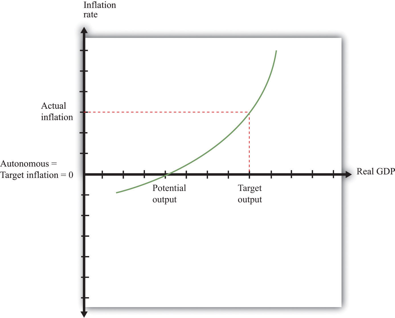
If target inflation = autonomous inflation = 0, but target output is above potential output, then the Fed will reduce the real interest rate and create more output to meet its target output. This will create inflation.
This is not the end of the story. Everyone in the economy is predicting zero inflation, yet the Fed is using its monetary policy to increase output and create positive inflation. Over time, people will notice that their expectations are wrong and will start to expect positive inflation instead. This results in an increase in autonomous inflation and a shift in the relationship between inflation and output.
At that point the Fed will have an incentive to create still more inflation to pursue its goal of output above potential. But additional inflation is costly to the Fed because it is now moving away from its target of zero inflation. Eventually inflation will be so high that the Fed no longer wants to create more inflation to increase output. The economy will end up with a positive inflation rate, where expectations of inflation are equal to actual inflation and no one is fooled. In the end, the Fed incurs an inflation rate above its target, yet it does not succeed in creating output above potential.
The final outcome involves costly inflation, but output remains at potential. Given that it cannot actually keep output above potential, the Fed would prefer zero inflation, yet it lacks the ability to commit to a zero-inflation policy. If the inflation rate is zero, the Fed has an incentive to create positive inflation.
The Politics of Fiscal Policy
The government budget constraint tells us that are three ways to fund spending: taxes today, the inflation tax, or debt (which means taxes at some future date). A government that has the best interests of its citizens at heart will decide on the best mix of these three. Optimists may believe that this is what governments try to do. Cynics might hold a very different view. Suppose—just suppose—that the leader of a government is more concerned with reelection than with sound economic policy and believes that her chances of reelection will be increased if she pledges not to increase taxes now or in the future. If this promise is credible, then the government budget constraint tells us that any increases in spending must be financed by money growth.
The monetary authority again has no power to commit to avoid inflation. The fiscal side of the government has set the level of spending and decided, based on the wishes of the political leaders, to have low taxes. Faced with this fiscal package, the monetary authority has no choice: it must print money to finance the government budget constraint. This story relies on the belief that individuals in the economy do not understand that the government, by its fiscal actions, is causing inflation and thus imposing a kind of tax.
A more extreme example arises when the government’s expenditures are so great that it simply cannot finance them with current taxation. This can occur in poorer economies where the tax base is low and the mechanisms for collecting taxes are often imperfect. Moreover, a government can finance its deficit through borrowing only if the public is willing to purchase government bonds. If a government is in fiscal trouble—if its tax and spending policies appear to the public to be unsustainable—it will have great difficulty persuading the public and the international investment community to buy government debt. Investors will demand a very high interest rate (including a risk premiumA part of the interest rate needed to compensate the lender for the risk of default.) to cover the possibility that the government may default on its debt. Interest rates on debt will increase.
At this point a government may find that the only option available to it is to finance its deficit through the printing of money. After all, no government wants to be in the position of being unable to pay its soldiers. The leaders of a country in such a position will decide to run the printing presses instead. The end result is inflation and, if the process gets completely out of control, hyperinflation. But from the government’s point of view, at least it buys it some time. Thus although moderate inflations are caused by poor monetary policy, hyperinflations are almost always originally caused by unsustainable fiscal policies.
Regional Monetary Policy
Figure 26.10 "The Price Level in Argentina" shows the price level in Argentina from 1988 to 2005. Argentina experienced hyperinflation in the early 1990s. Prices were then stable for about a decade and then increased again in the early years of the 21st century. In Argentina, different regional governments have significant power over the decisions of the central government. (It is as if a state government in the United States could appeal for funds directly from Washington.) These transfers from the central government in turn must be funded either from tax revenues or by printing money. If a region is sufficiently powerful relative to the central government, then it is as if the regional government has the power to print currency.
Figure 26.10 The Price Level in Argentina
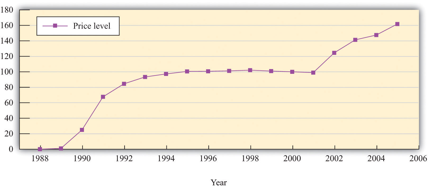
Source: International Monetary Fund World Economic Outlook database (http://www.imf.org/external/pubs/ft/weo/2010/01/index.htm).
A battle between regional governments can give rise to hyperinflation.Russell Cooper and Hubert Kempf, “Dollarization and the Conquest of Hyperinflation in Divided Societies,” Federal Reserve Bank of Minneapolis Quarterly Review, Summer 2001, accessed July 21, 2011, http://www.minneapolisfed.org/research/QR/QR2531.pdf. To simplify the issue, suppose that each region in Argentina has its own printing press. Each region can then independently undertake monetary policy by printing Argentine pesos and using those pesos to fund projects within their regions. The inflation tax is very tempting in these circumstances: a regional government can in effect tax people in other regions to help pay for its own projects. Why? Because printing money results in an inflation tax on everyone who has pesos. If money is printed in one region, some of the inflation tax will be paid by people in other regions who have pesos.
To be concrete, imagine you are a politician in Buenos Aires who wants to raise 100 million pesos for a project in that city. You could levy an income tax on citizens of your area. Alternatively, you could print 100 million pesos. If you impose the income tax, your own citizens must pay it all. If you impose the inflation tax, people living in other regions of Argentina pay some of the tax. Your constituents get the benefit, but others bear a large part of the costs. Acting in the interests of your constituents, you print the pesos. Of course, this story is true not only for you but also for the leaders in all regions. In the end, there is excessive money growth in the economy as a whole and high inflation. The monetary authorities are weak because no single authority controls the overall money supply.
The situation we have described is sometimes called a prisoners’ dilemmaThere is a cooperative outcome that both players would prefer to the Nash equilibrium of the game.. In a prisoners’ dilemma, the actions of one person imposes costs on others, and the behavior that is best for each individual decision maker (in this case, all the regional monetary authorities) is not best for the country as a whole.
Toolkit: Section 31.18 "Nash Equilibrium"
If you are interested in more detail on the prisoners’ dilemma game, you can review it in the toolkit.
Reducing Distortions from Taxes
Suppose a government faces a large expense today and can tax labor income to pay for it. One option is to increase income taxes today by a lot to finance this expense. This would cause a reduction in labor supply and thus in employment and real gross domestic product (GDP). This distortion in labor supply is an economic cost of the tax. Alternatively, the government could increase taxes a little bit today and a little bit in future years. This spreads out the tax over many years and leads to less distortion. The government budget constraint tells us that the government can spread out taxes by borrowing new and levying taxes later to pay off the debt.
If the government had access to a nondistortionary tax instead of income taxes, it would be better to use that tax instead. For a tax not to be distortionary, it must be the case that economic decisions (how much to buy and sell, how much labor to supply, etc.) do not change when the tax changes. At first glance, it seems that the inflation tax might fit the bill. Remember the inflation tax makes people’s existing stocks of money worth less in real terms. People have already decided how much money to hold. So if the government levies an inflation tax, it is not distortionary; people have already made their decisions on how much money they want to own.
But there is a danger here. Our argument rests on the idea that the decisions about which assets to hold have already been made by households. The inflation tax might be nondistortionary the first time that the government tried it. But people would rapidly come to anticipate that the government would be likely to use it again. At that point they would start changing their decisions about how much money to hold, and the tax would be distortionary after all.
Key Takeaways
- A government that prints money to finance its deficit is using an inflation tax. Individuals who hold nominal assets such as currency pay the tax.
- One source of inflation is a commitment problem of a central bank wishing to use inflation to boost output.
- When there are multiple regions (states or countries) each with the power to print money, then inflation will tend to be higher than it would be if only a single central bank controlled the money supply.
Checking Your Understanding
- When you pay the inflation tax, do you have to fill out a form? If not, then how is the inflation tax collected?
- If a government has a deficit of $400 billion and sells $200 billion in debt, how much must it increase the money supply so that the government budget constraint holds?
26.4 The Costs of Inflation
Learning Objectives
After you have read this section, you should be able to answer the following questions:
- What are the costs of an excessive inflation tax?
- When does inflation cause a redistribution?
At the beginning of this chapter, we highlighted President Ford’s campaign to “Whip Inflation Now.” It is clear from that episode that even relatively moderate inflation is perceived as a bad thing. It is even more self-evident that massive inflations, such as those in Germany or Zimbabwe, are highly disruptive. It is hardly surprising that the stated primary objective of most central banks is price stability. All that said, we have not yet really explained exactly why inflation is costly.
An Excessive Inflation Tax
Inflation, used as one tax among many, may be an efficient way of raising some of a government’s revenues. The effects of the inflation tax are like the effects of any tax: people respond by substituting away from the activity being taxed. When the government taxes cigarettes, people smoke less. When the government taxes income, people work less. When the government taxes the money people hold, people hold less money. These changes in behavior are the distortions caused by taxation. People substitute away from holding money in two ways: (1) during moderate inflations, people allocate more of their time to transactions; and (2) during high inflations, people may cease using money altogether.
During high inflations, the real value of money decreases quickly. So if you work and get paid in money, you had better go shopping quickly to make purchases. During hyperinflations, people may literally spend more time trying to get rid of their money than they do earning it in the first place. The same distortion applies, although less dramatically, in times of low to moderate inflation. People respond to inflation by carrying less cash, on average. To do so, they must spend more time standing in line in the bank and at automatic teller machines.
Imagine that ice cream were to be used as money. In a very cold climate, ice cream is just fine as a store of value. In a very hot climate, by contrast, ice cream is a bad store of value. You would probably want to get paid every day, and as soon as you received your ice cream, you would run to the store to buy other goods and services before your money melted. You and everyone else would spend much more time shopping and less time working. Melting ice cream, in this world, is like inflation.
There is a good reason why we do not use ice cream as a medium of exchange. Because it is such a bad store of value, people would quickly abandon it in terms of some other way of trading. During hyperinflations, this is exactly what we see: people substitute away from money completely and instead resort to barter trades. Often, some other commodity, such as cigarettes, starts being generally accepted as an alternative to money. But substitution away from money is costly to the economy. Money facilitates trade. It is generally easier to trade when everyone uses money rather than goods in exchange. When people respond to high inflation by eliminating money from trades, we are observing a distortion from the inflation tax.
Uncertainty and Real Interest Rates
It is the real interest rate that ultimately matters for saving and investment decisions. Yet loans are almost invariably quoted in nominal terms: a loan contract gives the borrower some money with a requirement to pay back that money plus interest in the future. The real and the nominal interest rates are linked by the Fisher equation:
real interest rate ≈ nominal interest rate − inflation rate.To calculate the real interest rate you subtract the inflation rate from the nominal interest rate. So, for example, if the annual interest rate on a car loan is 12 percent and the current inflation rate is 4 percent, then the real interest rate on the car loan is 8 percent.
Toolkit: Section 31.25 "The Fisher Equation: Nominal and Real Interest Rates"
You can review the derivation and uses of the Fisher equation in the toolkit.
The Fisher equation glosses over an important point, however. Suppose you are thinking of taking out a loan this year, allowing you to borrow money now for repayment next year. The inflation rate that matters for this loan is the inflation between this year and next. At the time you sign the contract, you do not know what the inflation rate will be. You must make your decision about the loan without knowing for sure what the real interest rate will be. You have to make a guess:
expected real interest rate ≈ nominal interest rate − expected inflation rate.Thus when a loan contract is signed, it is based on expectations of what will happen to prices in the future. If a borrower and lender would like to agree on a loan at a 4 percent real interest rate, but both expect 2 percent inflation, then they will agree on a 6 percent nominal interest rate.
What happens if the inflation rate turns out to be different from what the borrower and lender expected? Suppose the actual inflation rate turns out to be 4 percent. This means that the actual real interest rate, from the Fisher equation, is only 2 percent. This is good news for the borrower: he gets a loan at a lower rate than he expected. But it is bad news for the lender: she is repaid at a lower rate than she expected. The opposite is true if the inflation rate is lower than expected. Suppose the actual inflation rate is only 1 percent. Then the real interest rate is higher than anticipated—5 percent instead of 4 percent—which benefits the lender but is costly to the borrower.
Any divergence between actual and expected inflation therefore leads to a redistribution, either from the borrower to the lender or from the lender to the borrower. When inflation is higher than expected, the borrower is better off, and the lender is worse off. The opposite effects occur if inflation is lower than expected: the borrower loses, and the lender wins.
The possibility that the inflation rate will turn out to be unexpectedly high or unexpectedly low means that there is uncertainty whenever people sign loan contracts. A fixed nominal interest rate on a loan exposes both the borrower and the lender to the risk of inflation uncertainty. Uncertainty can prevent beneficial trades from taking place. Imagine that you were thinking of buying a used car, but you had to decide to buy without knowing whether the price was going to be $1,500 or $2,000. You might well decide not to buy in the face of this uncertainty. Similarly, people might sometimes decide not to sign loan contracts that would actually be beneficial to them.
The borrower and the lender could always change the form of their contract. Contracts do not have to specify nominal interest rates, and not all of them do. Some loans have interest rates that change with the actual inflation rate. In this way, borrowers and lenders can protect themselves from unexpected inflation. However, such contracts are unusual in practice and are most often seen in countries experiencing high and uncertain inflation. What should we conclude from the fact that loan contracts are rarely protected against inflation? Presumably one of two things is true: either such contracts are expensive to write or the benefit of these contracts is actually small.
Unexpected inflation can also have redistributive effects with other types of contracts. Labor contracts are an example. Although the worker and the firm ultimately care about real wages, most labor contracts are written in terms of nominal wages. That is, most labor arrangements are not indexed and thus leave the parties open to the effects of unanticipated inflation. So, for example, if inflation is higher than anticipated, then the real wage earned by the worker is lower than expected, which is a benefit to the firm.
Economies do respond to inflation, partly through the way in which people write contracts. In countries with high and volatile inflation, labor and other contracts generally provide some form of protection against inflation through indexation. For example, if you agree to a job that pays you $10 an hour this year, the nominal wage rate next year will change depending on inflation. If, for example, inflation was 20 percent this year, then under an indexed contract your nominal wage would automatically increase by 20 percent to $12. Under full indexation, the real wage you are paid is constant.
Key Takeaways
- Inflation can distort choices, such as the holding of money. A small amount of inflation, so that it is one tax among many, makes economic sense, but high inflation leads to significant distortion in the economy.
- Expected inflation is reflected in the terms of loan agreements. Unexpected inflation leads to a lower real interest rate and thus a redistribution from the lender to the borrower.
Checking Your Understanding
- If the inflation rate is lower than expected, who gains and who losses?
- What costs of inflation are highlighted in our discussion of Zimbabwe in Section 26 "Zimbabwe"?
26.5 Policy Remedies
Learning Objectives
After you have read this section, you should be able to answer the following questions:
- What actions can governments take to prevent excessive inflation?
- How can hyperinflations be ended?
- How do governments overcome the commitment problem?
We have already explained that money is a fragile social institution: money has value only because people believe it has value. Hyperinflations illustrate this fragility. Large inflations are impressive but, fortunately, are also relatively rare. In other words, most of the time monetary authorities are somehow able to maintain confidence in the system. To understand how they do so, we begin by looking at how hyperinflations come to an end.
Ending Big Inflations
As noted in Section 26.3.1 "The Inflation Tax", the rapid inflation in Germany ended abruptly. Although October 1923 was the month with the highest inflation rate, prices actually decreased in early 1924.
How did the hyperinflation end? The answer has to do with the conduct of fiscal policy. On October 15, 1923, a decree created a new currency from the old one. A key element of the decree was limits imposed on the money creation process by the central bank, particularly the provision of credit to the government. According to economist Thomas Sargent, who has studied how hyperinflations end, “This limitation on the amount of credit that could be extended to the government was announced at a time when the government was financing virtually 100 percent of its expenditures by means of note issue.”Thomas Sargent, “The Ends of Four Big Inflations,” in Inflation: Causes and Effects, ed. Robert Hall (Cambridge, MA: National Bureau of Economic Research, 1982), 83. Prior to October 1923, government spending was financed by printing money. After the decree, the printing presses were effectively turned off. As a consequence, the government’s budget went into surplus starting in January 1924. The hyperinflation was over once the printing presses were quiet.
Other countries that experienced hyperinflation around this time had similar stories: there was an abrupt end to hyperinflation after a regime change in which fiscal imbalances were restored. In Austria, for example, the inflation ended when the government established an independent central bank and adopted a fiscal policy that did not require financing by the central bank. The reforms in these countries had two effects: (1) the fiscal reforms limited the budget deficits, and (2) the monetary restrictions implied that deficits would not be financed by the printing of money.
A natural question is: what took them so long? Given the damage caused by these periods of hyperinflation, why did the countries not adopt these policies earlier? Part of the explanation may lie in political affiliations of the governments in these countries. Or, perhaps, these governments simply did not appreciate the rather complex links between fiscal and monetary policy.
Delegating Monetary Power to Another Country
Sometimes countries take even more drastic measures to shield monetary policy from political pressures. One is to effectively eliminate the monetary authority and delegate monetary policy to another country. Some small countries do this by simply using another country’s currency. Panama, El Salvador, and Ecuador, for example, have used the US dollar as their currency. Zimbabwe effectively did the same in 2009.
Argentina in the 1990s is an interesting example of a country that went almost—but not quite—that far. Figure 26.10 "The Price Level in Argentina" shows the price level in Argentina from 1988 to 2005. There are evidently three distinct periods: very high inflation, zero inflation, and then moderate inflation. From 1988 to 1993, there was substantial inflation. The annual inflation rate was about 343 percent in 1988 and was over 2,300 percent in 1990. But by 1993 it was only 10 percent, and from 1994 to 2001 it was effectively zero. Then, starting in 2002, there was a resurgence of inflation. What happened?
As we explained earlier, Argentina suffered from hyperinflation in the late 1980s as a consequence of a weak monetary authority. In 1991, Argentina adopted a novel monetary system called a currency boardA fixed exchange rate regime in which each unit of domestic currency is backed by holding the foreign currency, valued at the fixed exchange rate.. Every single peso in circulation was “backed” by a US dollar held by the Central Bank of Argentina. If desired, people had the right to take their pesos to the Central Bank of Argentina and swap them for dollars. Thus Argentina both adopted a fixed exchange rateA regime in which a central bank uses its tools to target the value of the domestic currency in terms of a foreign currency. between the peso and the dollar (1 peso equals $1) and also made that exchange rate credible by always having enough dollars on hand to exchange for the pesos in circulation. For all intents and purposes, Argentina had switched to using US dollars.
Argentina therefore avoided inflation by ceding control of monetary policy to the United States. Since the central bank in the United States controls the quantity of dollars and Argentina linked pesos to dollars, then, everything else the same, the Fed could change the amount of pesos in Argentina, whereas the Central Bank of Argentina could not. The Central Bank of Argentina could resist pressures to inflate by arguing that it did not control the money supply.
Many observers thought at the time that Argentina’s currency board would ensure price stability in Argentina. They thought that there would no longer be pressure on the monetary authority from the fiscal side of the economy. This proved to be incorrect. Taking advantage of its healthy economy in the early 1990s, Argentina adopted expansionary fiscal policies. A combination of factors then triggered recession in the country. Unemployment increased to 18 percent. It was not possible to expand fiscal policy much further, and Argentina had given up its control over monetary problem. In the late 1990s and early 2000s, the recession became so severe that the political pressure on the monetary authority was insurmountable. Argentina abandoned its currency board. One result was a resurgence of inflation.
Another variation on the delegation of monetary policy is that adopted by many countries in Europe. They decided to abandon their currencies and their monetary autonomy in favor of a new currency called the euro. Monetary policy is run by the European Central Bank, which is highly independent. Independent central banks are better able to resist political pressure, so countries that had previously had weak central banks saw a significant advantage in adopting the euro.
Abandoning one’s currency in favor of a new currency, as occurred throughout Europe, seems like a particularly powerful way for a country to commit to a new monetary regime. It is worth remembering, though, that no monetary system is cast is stone. Just as Argentina’s currency board collapsed despite its apparent credibility, so too could a country decide to abandon the euro and reestablish its own currency. Indeed, following fiscal problems in several countries in Europe (most notably Greece, Portugal, and Ireland), there has been some speculation that some countries might eventually choose to do just that.
Independent Monetary Authorities
Hyperinflations arise when the central bank is weak and unable to resist the pressures put on it by others—notably politicians—to use monetary policy for other purposes. Monetary authorities must be able to “just say no.” This suggests that monetary authorities will be able to do a better job if they are independent of other branches of government.
Economists have studied the relationship between measures of the independence of a country’s central bank and the inflation rate in that country. Economists Alberto Alesina and Lawrence Summers examined both political and economic independence of the monetary authority. By political independence, they meant the process of appointing the leadership of the central bank and the role of government officials in the conduct of monetary policy. By economic independence, they meant the extent to which the monetary authority is under pressure to finance the government’s budget deficit.
Figure 26.11 "Central Bank Independence and Inflation" displays data from their research. The horizontal axis shows annual inflation, and the vertical axis is their index of central bank independence, with higher numbers indicating a more independent central bank. The data are averaged over the period 1955–1988. Each point in the figure refers to a particular country. Switzerland and Germany both receive very “high” central bank independence ratings of 4 and have relatively low average inflation. Spain, in contrast, has the second lowest measure of central bank independence and has the highest inflation rate in the study.
Figure 26.11 Central Bank Independence and Inflation
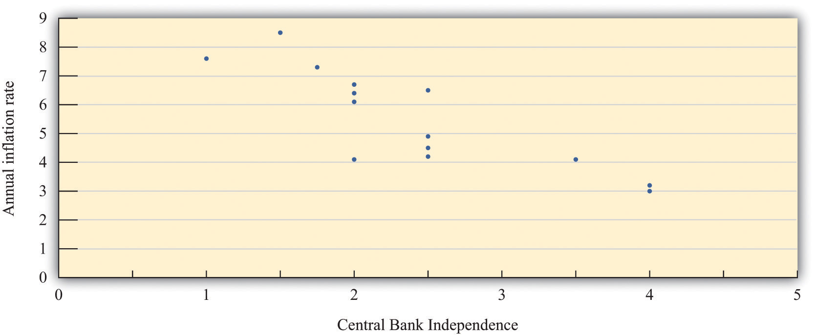
Since the work of Alesina and Summers (and other economists), more and more countries have become convinced of the virtues of having an independent central bank. For example, when the Labour Party came to power in Britain during the 1990s, one of their first acts was to make the Bank of England more independent. This was particularly striking because the Labour Party is a center-left political party, yet independent central banks tend to be conservative, focusing primarily on inflation and not worrying so much about employment and output.
Events in Argentina also attest to the value of an independent central bank. In 2003, the Congress in Argentina passed an act stating,
The Argentine Central Bank is a National State self-governed institution, whose primary and fundamental mission is to preserve the value of the Argentine currency.
When formulating and implementing the monetary and financial policy, it is not subject to the orders, guidelines or instructions of the National Executive branch of government.“BCRA Law,” Banco Central de la República Argentina, accessed September 20, 2011, http://www.bcra.gov.ar/institucional/in010000_i.asp.
There are two key elements in this act. First, the stated goal of the Central Bank of Argentina is to preserve the value of the currency. There is no mention of pursuing full employment, just a version of price stability. Second, the central bank is to be independent of the executive branch of the government.
Inflation Targeting
Under a policy regime called inflation targetingA regime in which the central bank uses its tools to set the inflation rate as close as possible to a target., some central banks use their tools to set the inflation rate as close as possible to a target. Just as we know that a monetary authority cannot literally control interest rates, we know it cannot literally set the inflation rate either. Rather, it can use the policy tools at its disposal to influence the economy in an attempt to reach the target inflation rate.
In its simplest form, the target is some publically announced inflation rate—say, 3 percent. If the monetary authority thinks the inflation rate is likely to be higher than 3 percent for the year, it adopts contractionary monetary policy to reduce the inflation rate. If it thinks that the inflation rate is likely to be lower than the target, it adopts an expansionary policy. Inflation in this world is relatively predictable.
What should the target be? If, as one might believe from all the discussion in the press and elsewhere, inflation is a pernicious problem, then perhaps the inflation target should be zero. Yet most central banks following this policy adopt targets with positive inflation rates, based on the belief that a little bit of inflation may be useful in the economy. One argument often heard is that deflation (negative inflation) is problematic. From a historical perspective, a prolonged period of deflation in the Unites States occurred during the Great Depression and coincided with a negative output growth. More recently, Japan experienced both slow real gross domestic product (real GDP) growth and some periods of deflation during the 1990s.
Many policymakers have apparently concluded that deflation is to be avoided because it could underlie a depression. An alternative possibility is that deflation is correlated with periods of low economic activity, but it is unclear whether it is the cause or the consequence of a sluggish economy. Whatever the connection between deflation and depression, the prevailing wisdom of the Fed (and other central banks) is to avoid deflation. Given that the central banks cannot always hit their targets precisely, aiming for zero inflation makes deflation more likely than when central banks adopt a target with positive inflation.
In addition, a little inflation may make it easier for relative prices and wages to adjust in an economy. If the demand for beef decreases and the demand for pork increases, then the price of beef should decrease, and the price of pork should increase. Such adjustment is straightforward. Similar logic says that if the demand for accountants decreases and the demand for systems analysts increases, then the wages of accountants should decrease, and the wages of systems analysts should increase. This may be more problematic. People typically respond very negatively if there is an attempt to cut their wages. It may be easier for employers to let inflation do the job of reducing the real wage instead. (This is an argument that makes some economists uncomfortable since it implies irrationality on the part of workers. Still, the psychological resistance to nominal wage cuts appears to be strong.)
A second issue is whether the inflation target should be allowed to vary. Instead of announcing a 3 percent target for all times, the monetary authority might decide that the target rate should depend on the state of the economy. For example, they could have a higher target rate in recession and a lower target rate in booms. This way monetary policy could still be used to help keep the economy at potential output.
Finally, there is the question of “punishment” for missing a target. If the purpose of inflation targeting is to support a particular (moderate) inflation rate, then a central banker missing the target ought to be fined or even terminated, just like a manager of a store who persistently misses sales targets. Presumably, if a central bank has goals to achieve, it should also have incentives to meet those goals. Central bankers are often called to testify in front of bodies, such as the US Congress, who monitor the progress of the economy relative to particular targets.
Australia is an example of a country that follows an inflation target rule. According to the charter of the Reserve Bank of Australia (http://www.rba.gov.au/monetary-policy/about.html), the goal of Australian monetary policy is to maintain inflation between 2 and 3 percent annually, on average. The central bank does also recognize of the role of monetary policy for stabilization purposes. Thus even though it has a target range for inflation, it also examines the state of the economy when setting monetary policy. Moreover, the phrase on average means that the central bank has some leeway in the conduct of policy: they can allow inflation to increase above 3 percent for a short while, provided that they eventually take actions to bring the inflation rate back down.
Key Takeaways
- Governments can take a variety of actions to prevent excessive inflation. These include the delegation of monetary policy to another central bank, the creation of an independent monetary authority, and constraining monetary policy to focus solely on inflation.
- Historically hyperinflations ended when the government restored fiscal balance by eliminating deficit spending.
- A government can overcome a commitment problem by delegating the conduct of monetary policy to a more conservative central bank. This can be achieved through a currency board or through joining a monetary union.
Checking Your Understanding
- What is the difference between a fixed exchange rate and a currency board?
- What is an independent central bank?
26.6 End-of-Chapter Material
In Conclusion
We have studied some severe and extreme cases of inflation to reveal the sources of rapid price increases. The quantity equation and the data both clearly indicate that inflation is linked to money supply growth. During periods of rapid inflation, the money supply is growing as well. The velocity of money also increases in times of rapid inflation, reflecting the collapse of confidence in the monetary system.
Money supply growth, in turn, comes about because money creation can help finance government budget deficits. Instead of using taxes to finance government spending, governments just print money. This increases prices and thus acts like a tax on those holding money and other nominal assets. Like all taxes, the inflation tax is distortionary. Used in moderation, there is an argument for using this tax along with others. But for some countries in some time periods, the use of the inflation tax has been excessive and there have been very costly hyperinflations.
The way to avoid excessive inflation is to create fiscal balance and monetary discipline. The big inflations between World War I and World War II ended when fiscal balance was restored. Monetary discipline comes in many forms. It requires an independent central bank, immune from political pressures. It may also require a central bank focused on an inflation target, paying less attention to other macroeconomic issues.
Key Links
- PBS history of German hyperinflation: http://www.pbs.org/wgbh/commandingheights/shared/minitext/ess_germanhyperinflation.html
- Federal Reserve releases on the measures of the money stock: http://www.federalreserve.gov/releases/h6
- International Monetary Fund country report on Zimbabwe: http://www.imf.org/external/pubs/ft/scr/2011/cr11135.pdf
- Australia Monetary Policy: http://www.rba.gov.au/monetary-policy/about.html
- Jim Bullard, Federal Reserve Bank president, Seven Faces of “the Peril”: http://research.stlouisfed.org/publications/review/10/09/Bullard.pdf
- Gary Stern, Federal Reserve Bank president, on deflation: http://www.minneapolisfed.org/research/pub_display.cfm?id=3354
- Federal Reserve Bank of Minneapolis publication on deflation: http://www.minneapolisfed.org/publications_papers/pub_display.cfm?id=3350
Exercises
- What is the difference between the quantity equation and the quantity theory of money?
- According to the classical dichotomy, what happens to the real money supply if the nominal money supply grows at 10 percent?
- If you were to draw a line through the points in Figure 26.6 "Inflation and Money Growth in Different Countries", it would not pass through the origin. Can you explain why? (Hint: examine the equation for the quantity equation, expressed in growth rates.)
- Looking at Figure 26.10 "The Price Level in Argentina", you might be fooled into thinking that the inflation between 2002 and 2003 was almost as bad as that between 1990 and 1991. Why would this reasoning be a mistake?
- The chapter contains two perspectives on Germany. The first is the hyperinflation in Germany during the 1920s, and the second is current Germany with low inflation and an independent central bank. How would you describe the differences in economic achievement (inflation, output growth, and unemployment) between these two versions of Germany? What were the institutional differences between these two versions of Germany?
- Looking at Table 26.2 "The Start of the Hyperinflation in Zimbabwe", what happened to the velocity of money in Zimbabwe during the hyperinflation?
- If the central bank takes the view that producing at potential GDP is efficient, then does it face a commitment problem?
- In 2010, the state of California faced severe budgetary problems. If the state could print dollars, how would that relieve its budget problems? Who would pay the inflation tax?
Economics Detective
- In the United States, how many central banks are there?
- In note 5, we mention a measure of the money supply called “M2.” There are other measures of the money supply. For example, “M1” refers to currency and other assets that are immediately available for spending purposes. Find the most recent measure of the stocks of M1 and M2 for the United States.
- Calculate the velocity of money for a country other than the United States.
- The chapter did not present data on other recent periods of high inflation in countries such as Argentina, Brazil, Israel, and others. Search the Internet to find data on the inflation experiences of these countries. Create a graph of the growth rates of inflation and money in one of these countries.
- It might be that countries have high money growth and thus high inflation because these are the goals of their monetary authority. See whether you can find a monetary authority with a stated goal of high inflation. If not, then think about why countries experience inflation if that is not the objective of the monetary authority?
- What countries are dollarized in the world economy? Try to find out how dollarization influenced the inflation rate in that country.
- Try to find a statement of the objectives of the Central Bank of Argentina. Part of independence is the way in which the decision makers at the central bank are appointed. How are these appointments made in Argentina?
- Go to the web page for the Bank of Australia to learn about inflation targeting. What is their inflation target? How is it determined? What happens if they miss the target? Compare this to the objective and policy decisions of the Fed in the United States. What other central banks follow an inflation-targeting rule?
- Is monetary policy in the United States guided by an inflation target? Does the European Central Bank use an inflation target?
Spreadsheet Exercise
- Create a version of Table 26.1 "Prices in Germany" using a spreadsheet. Examine quarterly data for the United States or another country for the years 2007 to 2009. For prices, use the GDP implicit price deflator. Use the spreadsheet to calculate the inflation rate. Then put in a measure of the money supply and real GDP. Use the spreadsheet to calculate the velocity of money. Is the velocity of money approximately constant?