This is “Job and Worker Flows”, section 23.2 from the book Theory and Applications of Economics (v. 1.0). For details on it (including licensing), click here.
For more information on the source of this book, or why it is available for free, please see the project's home page. You can browse or download additional books there. To download a .zip file containing this book to use offline, simply click here.


23.2 Job and Worker Flows
Learning Objectives
After you have read this section, you should be able to answer the following questions:
- What key features of labor markets does the static model of labor supply and labor demand fail to capture?
- What are some of the key facts about worker labor market flows?
- What is search theory, and how is it useful for understanding labor market outcomes?
- What are the efficiency gains from flexible labor markets?
The labor market is a highly dynamic place. Workers are constantly moving from job to job, in and out of the workforce, or from employment to unemployment and vice versa. Large firms devote substantial resources to human resource management in general and hiring and firing in particular. By contrast, Figure 23.4 "Unemployment in the Labor Market" is static because it shows the labor market at a moment in time. Our understanding of the labor market—and, by extension, employment and unemployment—is badly incomplete unless we look more carefully at the movement of workers. Further, when workers and firms meet, they do not take as given a market wage but instead typically engage in some form of bargaining over the terms of employment.
This vision of a dynamic labor market with bargaining is much closer to the reality of labor relations than is the model of labor supply and demand. To better understand the determinants of employment and unemployment, we therefore turn to labor market flows. We begin with some more facts, again contrasting the experience of Europe with that of the United States, and then develop a framework that allows us to think explicitly about the dynamic labor market.
Facts
Our starting point is the classification of individuals in the civilian working age population. Recall that economic statistics place them as one of the following: employed, unemployed, or not in the labor force. Imagine taking a snapshot of the US economy each month. For a given month, you would be able to count the number of people employed, unemployed, and out of the labor force. We could call these the stocks of each kind of individual.
Figure 23.5 Worker Stocks in the United States
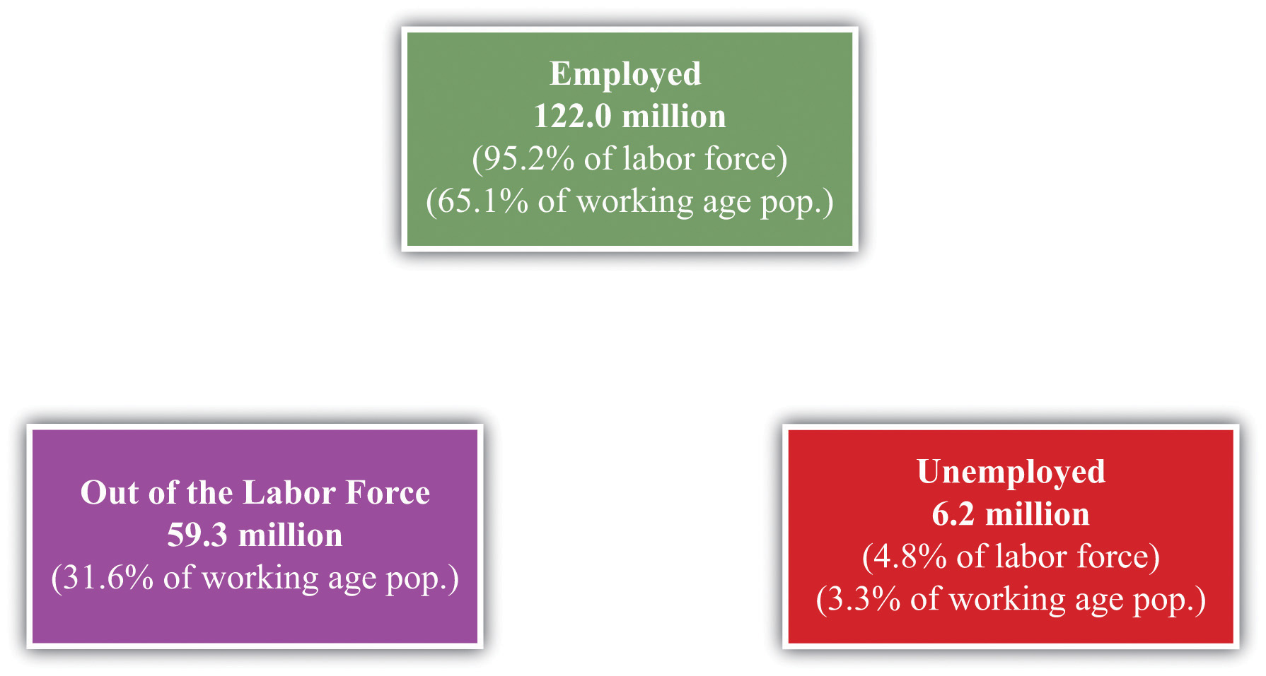
Figure 23.5 "Worker Stocks in the United States" shows the number of people between 16 and 64 years old in the United States in three different “states”—employment, unemployment, and out of the labor force—over the period 1996–2003.These data come from a study using a monthly survey conducted by the Bureau of Labor Statistics (BLS) called the Current Population Survey and were compiled by Stephen J. Davis, R. Jason Faberman, and John Haltiwanger. The numbers here come from S. Davis, R. J. Faberman, and J. Haltiwanger, “The Flow Approach to Labor Market: New Data Sources and Micro-Macro Links” NBER Working Paper #12167, April 2006, accessed June 30, 2011, http://www.nber.org/papers/w12167. On average, there were 122 million people employed, 6.2 million unemployed, and 59.3 million considered out of the labor force. Adding these numbers together, there were 187.5 million working-age individuals, of whom 128.2 million were in the labor force. The average unemployment rate was 4.8 percent over this period, and the employment rate was 95.2 percent. Notice, though, that many individuals are out of the labor force: only 65 percent of the population is employed.
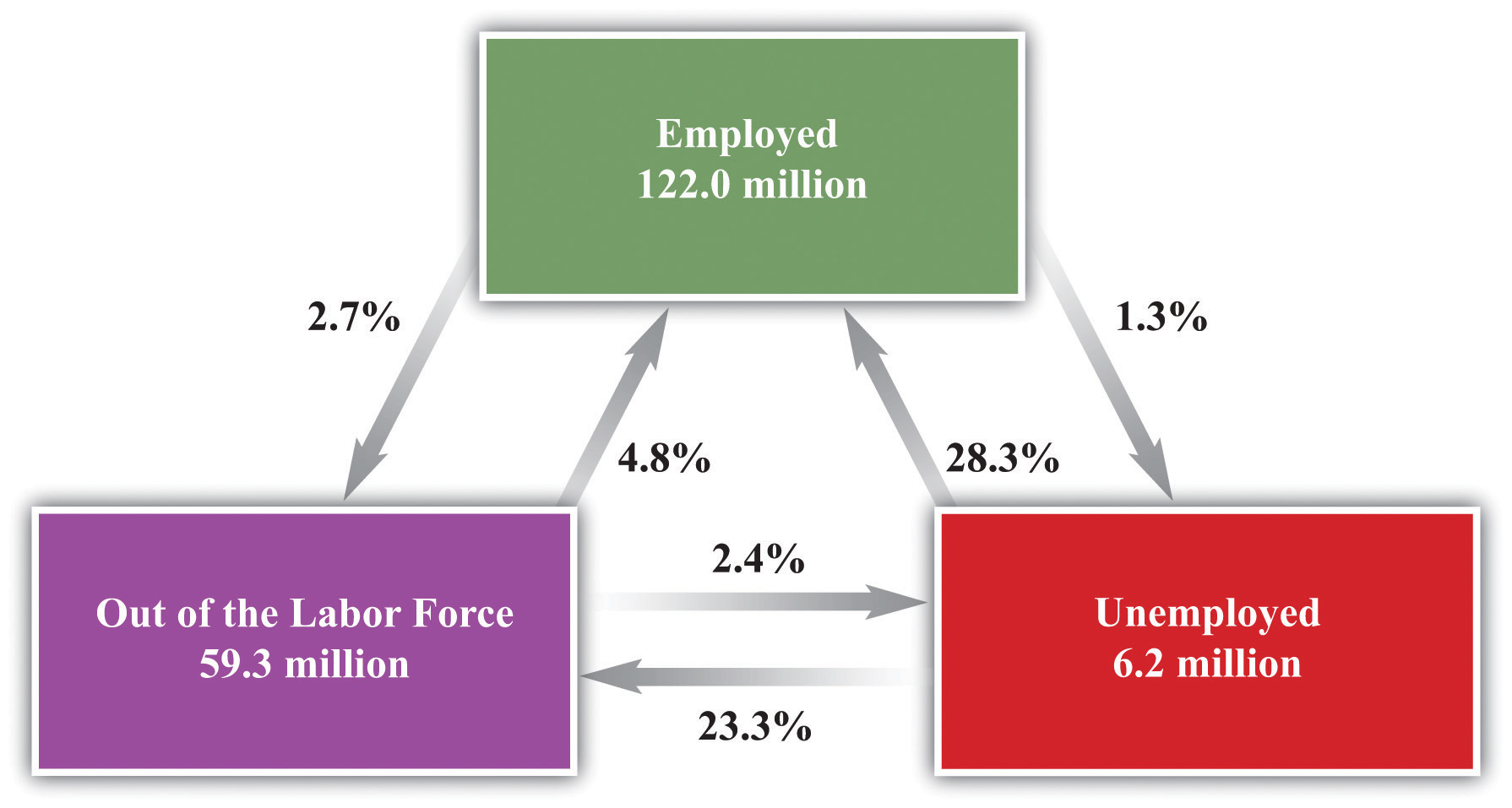
Figure 23.5 "Worker Stocks in the United States" shows an average over many months, but you could also look at how these numbers change from month to month. Even more informatively, you could count the number of people who were employed in two consecutive months. This would tell you the likelihood of being employed two months in a row. These calculations for the US economy are summarized in Figure 23.6 "Worker Flows in the United States".
Look, for example, at the arrows associated with the box labeled unemployed. There are two arrows coming in: one from the employed box and one from the out-of-the-labor-force box. There are two arrows going out: one to the employed box and one to the out-of-the-labor-force box. Each of these four arrows has a percentage attached, indicating the fraction of people going from one box to another. Thus, on average, 28.3 percent of the unemployed people in one month are employed in the next and 23.3 percent leave the labor force. The remaining 48.4 percent stay in the group of unemployed.
The numbers in the figure are averages over a long period. Such flows change over the course of the year due to seasonal effects. Around Christmas, for example, it may be easier for an unemployed worker to find a job selling merchandise in a retail shop. These flows also change depending on the ups and downs of the aggregate economy.
Figure 23.6 Worker Flows in the United States
Do European countries exhibit similar patterns? Portugal makes for a good comparison with the United States because the unemployment rates in the two countries were broadly similar over most of the last two decades. Yet Portugal has very strong employment protection laws, to the point where they are enshrined in the Portuguese Constitution:“Article 53,” Portugal-Constitution, adopted April 2, 1976, accessed June 30, 2011, http://www.servat.unibe.ch/icl/po00000_.html#A053_.
Article 53 Job Security
The right of workers to job security is safeguarded. Dismissals without just cause or for political or ideological reasons are forbidden.
A study that compared the labor markets in Portugal and the United States uncovered the following facts:See Olivier Blanchard and Pedro Portugal, “What Hides Behind an Unemployment Rate: Comparing Portuguese and U.S. Labor Markets,” American Economic Review 91, no. 1, (2001), 187–207.
- The flows into unemployment from employment and the flows from employment to unemployment are much lower in Portugal compared to the United States.
- Average unemployment duration in Portugal is about three times that of the United States.
- Job protection is very high in Portugal relative to the United States.
Even though Portugal and the United States have similar overall unemployment rates, the underlying flows are quite different in the two countries. Flows between employment and unemployment—and vice versa—are much smaller in Portugal. This means that if you lose your job, it is likely to take a long time to find a new one. If you have a job, you are likely to keep it for a long time. As we would expect from this, people typically spend much longer periods of time in unemployment in Portugal than they do in the United States.
If we compare the United States with Europe more generally, we see similar patterns. In 2010, the average unemployment durationThe amount of time a typical worker spends searching for a new job. for workers ages 15–24 was about 10.6 months in Europe but only 5.9 months for the United States. For workers in the 25–54 age group, the duration was higher in both Europe (13.7 months) and the United States (8.2 months) than for younger workers.See “Unemployment Duration,” Online OECD Employment database, accessed June 30, 2011, http://www.oecd.org/document/34/0,3746,en_2649_33927_40917154_1_1_1_1,00.html#uduration. Recall that in 2010, Europe and the United States had similar rates of unemployment. Employment duration, however, is still much higher in Europe than the United States. In both places, older workers tend to be unemployed for longer periods than younger workers. But European workers are typically unemployed for much longer periods of time than US workers.These figures come from “Average Duration of Unemployment,” OECD, accessed June 30, 2011, http://stats.oecd.org/Index.aspx?DataSetCode=AVD_DUR.
The Organisation for Economic Co-operation and Development (OECD) conducted a large study on the employment protection legislation in a variety of developed countries. The main study (OECD Employment Outlook for 2004, http://www.oecd.org/document/62/0,3746,en_2649_33927_31935102 _1_1_1_1,00.html) created a measure of employment protection and then attempted to relate it to labor market outcomes in different countries. The reasoning we have just presented suggests that in countries with relatively high levels of employment protection, labor markets would be much more sluggish.
Formulating a comprehensive measure of employment protection is not easy. In principle, the idea is to measure the costs of firing workers and various regulations of employment. Examples would include requirements on advance notice of layoffs and the size of severance payments that firms are obliged to pay. In some countries, a firm must go to court to lay off workers. For temporary workers, there are specific restrictions placed on this form of contract, as in the discussion of France that opened this chapter. In reality, these costs are difficult to detect and convert to a single measure. The OECD findings should be interpreted with these challenges in mind.
Another OECD publication (http://www.oecd.org/dataoecd/40/56/36014946.pdf) examines employment protection legislation across OECD countries in 1998 and 2003.This discussion is based on Figure A.6 of OECD, “Annex A: Structural Policy Indicators,” Economic Policy Reforms: Going for Growth, accessed June 30, 2011, http://www.oecd.org/dataoecd/40/56/36014946.pdf. Portugal was the country with the highest level of employment protection legislation, while the United States was the lowest. France was above average, while the United Kingdom and Canada were below average. The OECD analysis highlighted two effects of such legislation on labor market flows:
- It limits flows from employment into unemployment because it is costly to fire workers.
- It limits flows from unemployment to employment because firms, when deciding to hire a worker, will realize that they may wish to fire that worker sometime in the future.
The first effect is the more obvious one; indeed, it provides the rationale for employment protection. If it is hard to fire workers, then firms are less likely to do so. The second effect is less obvious and more pernicious. If it is hard to fire workers, then firms become more reluctant to hire workers. Put yourself in the place of a manager wondering whether to make a hire. One concern is that the person you are considering will turn out to be unsuitable, or a bad worker. Another is that conditions in your industry will worsen, so you may not need as many employees. In those circumstances, you want to be able to let the worker go. If you will not be able to do so, you may decide it is safer simply to make do with the workers you already have.
The OECD analysis particularly stressed the effects on the labor market experience of relatively young workers. The report emphasized that stronger legislation is linked to lower employment of young workers. If it is costly to sever a relationship, then a firm will not give a young worker a chance in a new job. The OECD also noted an important benefit of employment protection legislation: it enhances the willingness of young workers to invest in skills that are productive at their firms. Without a strong attachment to the firm, workers have little incentive to build up skills that are not transferable to other jobs.
Job Creation and Job Destruction
In place of the supply-and-demand diagram, we can think about the decisions that workers and firms make when they are trying to form or break an employment relationship. Individual workers search for available jobs, which are called vacancies. On the other side, vacancies are searching for workers. When a vacancy and a worker are successfully matched, a job is created. When we say that a vacancy is searching for a worker, we, of course, really mean that a firm with a vacancy is seeking to hire a worker. You can think of a firm as being a collection of jobs and vacancies.
Whereas the standard supply-and-demand picture downplays differences among workers and jobs, this “search-and-matching” approach places these differences at the center of the analysis. Workers differ in terms of their abilities and preferences. Jobs differ in terms of their characteristics and requirements. For an economy to function well, we need to somehow do a good job of matching vacancies with workers. When a successful match occurs, we call this “job creation.”
Search theoryA framework for understanding the flows of workers across periods of employment and unemployment along with the creation of job vacancies by firms. is a framework for understanding this matching process. Let us think about how this process looks, first from the perspective of the worker and then from the perspective of the firm. Workers care about the various characteristics of their jobs. These characteristics might include how much the job pays, whether it is in a good location, whether it offers good opportunities for advancement, whether it is interesting, whether it is dangerous, and other attributes.
Vacancies are likewise “looking” for certain characteristics of workers, such as how much they cost, what skills they possess, whether they have relevant experience, whether they are hardworking and motivated, whether they are trustworthy, and so on. The firm cares about these characteristics because it cares about profitability: its goal is to make as much profit as possible.
Over time, the quality of the match between a worker and a vacancy may change. A job may become less profitable to the firm and/or less attractive to the worker. To put it another way, the amount of value created by the job may change. The worker may come to dislike particular aspects of the job or may wish to change location for family reasons. The worker may feel that he or she would be better matched with some other firm, perhaps because of changes in his or her skills and experience. From the firm’s side, demand for the firm’s product may decrease, or the firm might shift to a new production technique that requires different skills. If the value created by a job decreases too much, then the firm or the worker may choose to end the relationship, either by the worker’s choice (quitting the job) or the firm’s (firing the worker). This is “job destruction.”
Jobs are created and destroyed all the time in the economy. The flows of workers among jobs and employment states are a key characteristic of the labor market. As these flows occur, workers often spend time unemployed. After a job is destroyed, the worker may spend some time unemployed until he or she finds a job with a different firm.
Labor Flows and Productivity
In a rapidly changing economy, the value of different jobs (worker-firm matches) changes over time. To function efficiently, the labor market needs to be able to accommodate such changes. For this discussion, we will think about efficiency as simply being measured by the productivity of the match between workers and firms. In an efficient match, the worker is productive at the chosen job. For the overall economy, if all matches are efficient, then it is not possible to change the assignment of workers to jobs and produce more output.
Comparative and Absolute Advantage
Let us see how this works in a simple example. Table 23.1 "Output Level per Day in Different Jobs" gives an example of an economy with two workers and two jobs. Each entry in the table is the amount of output that a particular worker can produce in each job in one day. For example, worker B can produce 4 units of output in job 2 and 8 units of output in job 1.
Table 23.1 Output Level per Day in Different Jobs
| Worker | Job 1 | Job 2 |
|---|---|---|
| A | 9 | 6 |
| B | 8 | 4 |
Before we begin, let us pause for a moment to think about this kind of example. This chapter is motivated by the desire to explain the employment and unemployment experiences of hundreds of millions of workers in the United States and Europe. It may seem ridiculous to think that a story like this—with two workers, two jobs, and some made-up numbers—can tell us anything about employment and unemployment across two continents. Economists often refer to such stories as “toy” models, in explicit recognition of their simplicity. This kind of model is not designed to tell us anything specific about US or European unemployment. The point of this kind of model is to keep our thinking clear. If we cannot understand the workings of a story like this, then we cannot hope to understand the infinitely more complicated real world. At the same time, if we do understand this story, then we begin to get a feel for the forces that operate in the real world.
If we were in charge of this economy, how would we allocate the workers across the jobs? In this case, the answer is easy to determine. If we assign worker A to job 1 and worker B to job 2, then the economy will produce 13 units of output per day. If we assign worker A to job 2 and worker B to job 1, then the economy will produce 14 units of output per day. This is the better option because—in the interest of efficiency—we would like the workers to be assigned to the jobs they do best.
Notice, by the way, that worker A is better than worker B at both jobs. However, worker A is a lot better at job 2 (50 percent more productive) and only a little better at job 1 (12.5 percent more productive). The best assignment of workers is an application of the idea called comparative advantage: each worker does the job at which he or she does best when compared to the other person.
Comparative advantageIn the production of one good, the opportunity cost, as measured by the lost output of the other good, is lower for that person than for another person. and absolute advantageIn the production of a good, one person can produce more of a good in a unit of time than another person. are used to compare the productivity of people (countries) in the production of a good or a service. We introduce this tool here assuming there are two people and two goods that they can each produce.
Toolkit: Section 31.13 "Comparative Advantage"
A person has an absolute advantage in the production of a good if that person can produce more of that good in a unit of time than another person can. A person has a comparative advantage in the production of one good if the opportunity cost, measured by the lost output of the other good, is lower for that person than for another.
In our example, worker A has a comparative advantage in job 2, and worker B has a comparative advantage in job 1. We have defined comparative advantage in terms of opportunity costWhat you must give up to carry out an action., so let us go through this carefully and make sure it is clear. The opportunity cost of assigning a worker to one job is the amount of output the worker could have produced in the other job.
We can measure opportunity cost in terms of the output lost from assigning a worker to job 2 instead of job 1. The opportunity cost of assigning worker A to job 2 rather than job 1 is 3 units (9 − 6). The opportunity cost of assigning worker B to job 2 rather than job 1 is 4 units of output (8 − 4). The opportunity cost is higher for worker B, which is another way of saying that worker B has a comparative advantage in job 1. Worker B should be assigned to job 1, and worker A should take on job 2.
We could equally have measured opportunity cost the other way around: as the output lost from assigning a worker to job 1 rather than job 2. The opportunity cost of assigning worker A to job 1 rather than job 2 is −3 units (6 − 9). The opportunity cost of assigning worker A to job 1 rather than job 2 is less, it is −4 units of output (4 − 8). Worker A has the higher opportunity cost (−3 is greater than −4), so we again conclude that worker A should be assigned to job 2.
Changes in Productivity
Suppose that this simple economy is indeed operating efficiently, with worker A in job 2 and worker B in job 1. Then imagine that the productivity of one of these matches changes. For example, suppose that at some point worker B goes on a training course for job 2, so Table 23.1 "Output Level per Day in Different Jobs" becomes Table 23.2 "Revised Output Level per Hour from Assigning Jobs".
Table 23.2 Revised Output Level per Hour from Assigning Jobs
| Worker | Job 1 | Job 2 |
|---|---|---|
| A | 9 | 6 |
| B | 8 | 7 |
If you compare these two tables, you can see that worker B is now more productive than worker A in job 2. Worker A is still better at job 1, as before.
If we want to produce the maximum amount of output in this economy, we now want to switch the workers around: if worker A does job 1 and worker B does job 2, then the economy can produce 16 units of output per day instead of 14.
How might this change happen in practice? Here are three scenarios.
- Instantaneous reallocation. In this case, the labor market is very fluid. Workers A and B trade places as soon as B becomes more productive. No one is unemployed, and real gross domestic product (real GDP) increases immediately.
- Stagnant labor market. This scenario is the opposite of the first. Here, there is no reallocation at all. People are stuck in their jobs forever. In this case, worker B remains assigned to job 1, and worker A remains assigned to job 2. Although this was the best assignment of jobs when Table 23.1 "Output Level per Day in Different Jobs" described the economy, it is not the best assignment for Table 23.2 "Revised Output Level per Hour from Assigning Jobs". Relative to the better assignment, the economy loses 2 units of GDP every day.
-
Frictional unemployment. This scenario lies between these two extremes: workers and firms adjust but not instantaneously. How might workers A and B exchange jobs? One possibility is that worker A is fired from job 2 because the firm wants to attract worker B to the job instead. At the same time, worker B might quit in the hope of getting job 1 when it is vacant. Both workers move from employment into unemployment, as in the arrow from employment to unemployment in Figure 23.6 "Worker Flows in the United States".
During the time when workers A and B are unemployed, their production is reduced to zero. So, during the period of adjustment, the economy in the third scenario undergoes a recession. But once adjustments are made, the economy is much more productive than before. Economists refer to the unemployment that occurs when workers are moving between jobs as frictional unemploymentThe unemployment that occurs when workers are moving between jobs..
How do these three scenarios compare? It is evident that fluid labor markets are the ideal scenario. In this situation, there is no lost output due to unemployment, and the economy is always operating in the most efficient manner. The choice between the second and third scenarios is not so clear-cut. In the second scenario, there is no loss of output from unemployment, but the assignment of workers to jobs is not efficient. In the third scenario, the economy eventually gets back to the most efficient assignment of jobs, but at the cost of some lost output and unemployment (and, in the real world, various other costs of transition incurred by workers and firms).
You can think of the time spent in unemployment in the second scenario as a type of investment. The economy forgoes some output in the short run to enjoy a more efficient match of workers and firms in the long run. As with any investment decision, we decide if it is worthwhile by comparing the immediate cost (the first four weeks of lost output) with the discounted present value of the future flow of benefits. Discounted present value is a technique that allows us to add together the value of dollars received at different times.
Toolkit: Section 31.5 "Discounted Present Value"
Discounted present value is a technique for adding together flows at different times. If you are interested in more detail, review the toolkit.
Suppose, for example, that it takes four weeks for the economy to reallocate the jobs in the third scenario. Assuming the workweek has 5 working days, the economy produces 0 output instead of 14 units of output for a total of 20 days. The total amount of lost output is 20 × 14 = 280. Once the workers have found their new jobs, the economy produces 10 more units per week than previously. After 28 weeks, this extra output equals the 280 lost units. If we could just add together output this month and output next month, we could conclude that this investment pays off for the economy after 28 weeks. Because output produced in the future is worth less than output today, it will actually take a bit longer than 28 weeks for the investment to be worthwhile.
Provided that changes to the relative productivity of workers do not occur too frequently, the costs of adjusting the assignment of workers to jobs (the spells of unemployment) will be more than offset by the extra output obtained by putting workers into the right jobs. This is the gain from a fluid labor market, even though the process entails spells of unemployment.
Youth Unemployment
We observed earlier that the unemployment rate for young workers is higher than for older workers, in both France and the United States. We can understand why by thinking about the search and matching process.
When lawyers, doctors, professors, and other professionals change jobs, they typically do so with little or no intervening unemployment. Search and matching is easy because they have visible records, meaning their productivity at a particular job is relatively easy to figure out. In general, the longer someone has been in the workforce, the more information is available to potential new employers. Also, experienced workers have a good understanding of the kinds of job that they like.
Just the opposite is more likely in the labor market for young workers. Firms know relatively little about the young workers they hire. Likewise, young workers, with little employment experience, are likely to be very uncertain about whether or not they will like a new job. The result, at least in the United States, is a lot of turnover for young workers. Young workers sample different jobs in the labor market until they find one suited to their tastes and talents. They take advantage of the fluid nature of the US labor market to search for a good match. The gain is a better fit once they find a job they like. The cost is occasional spells of unemployment.
In Europe, search and matching is much harder. Some young workers are even effectively guaranteed jobs for life by the government from the moment they finish college. By contrast, young workers without jobs find it difficult to obtain employment. Given the lack of fluidity in European labor markets, it is surprising neither that more young workers are unemployed, nor that they stay unemployed for longer periods of time.
The Natural Rate of Unemployment
We expect there to be some frictional unemployment, even in a well-functioning economy. We also know that there is cyclical employment associated with the ups and downs of the business cycle. When cyclical unemployment is zero, we say that the economy is operating at full employment. The natural rate of unemploymentThe amount of unemployment we expect in an economy that is operating at full employment. is defined as the amount of unemployment we expect in an economy that is operating at full employment—that is, it is the level of unemployment that we expect once we have removed cyclical considerations.
The natural rate of unemployment can seem like an odd concept because it says that it is normal to have unemployment even when the economy is booming. But it makes sense because all economies experience some frictional unemployment as a result of the ongoing process of matching workers with jobs. Government policies that affect the flows in and out of employment lead to changes in the natural rate of unemployment.
Key Takeaways
- The static model of labor supply and labor demand fails to capture the dynamic nature of the labor market and does not account for job creation and destruction.
- In the United States, labor markets are very fluid. Each month, a significant fraction of workers lose their jobs, and each month a significant fraction of unemployed workers find jobs.
- Search theory provides a framework for understanding the matching of workers and jobs and wage determination through a bargaining process.
- The economy is operating efficiently when workers are assigned to jobs based on comparative advantage. Inflexible labor markets lead to inefficient allocations of workers to jobs.
Checking Your Understanding
- Is it best to assign workers to jobs based on absolute advantage or comparative advantage?
- Why is frictional unemployment not always zero?