This is “What Happened during the Great Depression?”, section 22.1 from the book Theory and Applications of Economics (v. 1.0). For details on it (including licensing), click here.
For more information on the source of this book, or why it is available for free, please see the project's home page. You can browse or download additional books there. To download a .zip file containing this book to use offline, simply click here.


22.1 What Happened during the Great Depression?
Learning Objectives
After you have read this section, you should be able to answer the following questions:
- What are the main facts about the Great Depression?
- What is puzzling about the Great Depression?
- What are the two leading strands of thought about the cause of the Great Depression?
We begin with some facts. Table 22.1 "Major Macroeconomic Variables, 1920–39*" shows real gross domestic product (real GDP)A measure of production that has been corrected for any changes in overall prices., the unemployment rateThe percentage of people who are not currently employed but are actively seeking a job., the price levelA measure of average prices in the economy., and the inflation rateThe growth rate of the price index from one year to the next. from 1920 to 1939 in the United States. Real GDP measures the overall production of the economy, the unemployment rate measures the fraction of the labor force unable to find a job, the price level measures the overall cost of GDP, and the inflation rate is the growth rate of the price level.
Table 22.1 Major Macroeconomic Variables, 1920–39*
| Year | Real GDP | Unemployment | Price Level | Inflation Rate |
|---|---|---|---|---|
| 1920 | 606.6 | 5.2 | 11.6 | |
| 1921 | 585.7 | 11.7 | 10.4 | −10.3 |
| 1922 | 625.9 | 6.7 | 9.8 | −5.8 |
| 1923 | 713.0 | 2.4 | 9.9 | 1.0 |
| 1924 | 732.8 | 5.0 | 9.9 | 0.0 |
| 1925 | 748.6 | 3.2 | 10.2 | 3.0 |
| 1926 | 793.9 | 1.8 | 10.3 | 1.0 |
| 1927 | 798.4 | 3.3 | 10.4 | 1.0 |
| 1928 | 812.6 | 4.2 | 9.9 | −4.8 |
| 1929 | 865.2 | 3.2 | 9.9 | 0.0 |
| 1930 | 790.7 | 8.9 | 9.7 | −2.0 |
| 1931 | 739.9 | 16.3 | 8.8 | −9.3 |
| 1932 | 643.7 | 24.1 | 8.0 | −9.1 |
| 1933 | 635.5 | 25.2 | 7.5 | −6.3 |
| 1934 | 704.2 | 22.0 | 7.8 | 4.0 |
| 1935 | 766.9 | 20.3 | 8.0 | 2.6 |
| 1936 | 866.6 | 17.0 | 8.1 | 1.3 |
| 1937 | 911.1 | 14.3 | 8.4 | 3.7 |
| 1938 | 879.7 | 19.1 | 8.2 | −2.4 |
| 1939 | 950.7 | 17.2 | 8.1 | −1.2 |
| *GDP is in billions of year 2000 dollars (Bureau of Economic Analysis [BEA]). The unemployment rate is from the US Census Bureau, The Statistical History of the United States: From Colonial Times to the Present (New York: Basic Books, 1976; see also http://www.census.gov/prod/www/abs/statab.html). The base year for the price index is 2000 (that is, the index equals 100 in that year) and comes from the Bureau of Labor Statistics (BLS; http://www.bls.gov), 2004. | ||||
Looking at these data, we see first that the 1920s were a period of sustained growth, sometimes known as the “roaring twenties.” Real GDP increased each year between 1921 and 1929, with an average growth rate of 4.9 percent per year). Meanwhile the unemployment rate decreased from 6.7 percent in 1922 to 1.8 percent in 1926. Real GDP reached a peak of $865 billion in 1929. This number is expressed in year 2000 dollars, so we can compare that number easily with current economic data. In particular, if we divide by the population at that time, we find that GDP per person was the equivalent of about $7,000, in year 2000 terms. Real GDP per person has increased about fivefold since that time.
Toolkit: Section 31.21 "Growth Rates"
You can review growth rates in the toolkit.
The Great Depression began in late 1929 as a recession not unlike those experienced previously—a decrease in GDP from one year to the next was common—but it rapidly blossomed into a four-year reduction in economic activity. By 1933, real GDP had fallen by over 25 percent and was only $636 billion. At the same time, unemployment increased from around 3 percent to 25 percent. In 1929, jobs were easy to come by. By 1933, they were almost impossible to find. More than a quarter of the people wishing to work were unable to find a job. Countless others, no doubt, had given up even looking for a job and were out of the labor force.
The experience of the 1920s and 1930s tells us that when real GDP increases, unemployment tends to decline and vice versa. We say that unemployment is countercyclicalAn economic variable that typically moves in the opposite direction to real GDP, decreasing when GDP increases and increasing when GDP decreases., meaning that it typically moves in the direction opposite to the movement of real GDP. An economic variable is procyclicalAn economic variable that typically moves in the same direction as real GDP, increasing when GDP increases and decreasing when GDP decreases. if it typically moves in the same direction as real GDP, increasing when GDP increases and decreasing when GDP decreases. The countercyclical behavior of unemployment is not something that is peculiar to the Great Depression; it is a relatively robust fact about most economies. It is also quite intuitive: if fewer people are employed, less labor goes into the production function, so we expect output to be lower.
An event occurred in September 1929 that, at least with hindsight, marks a turning point. The stock market, as measured by the Dow Jones Industrial Average, had been increasing until that time but then decreased by 48 percent in less than 2.5 months. The value of the stock market is a measure of the value, in the minds of investors, of all the firms in the economy. Investors suddenly decided that the US economy was worth only half what they had believed three months earlier. It is unlikely that two such dramatic economic events occurred at almost the same time and yet are unconnected. We should not make the claim that the stock market crash caused the Great Depression. But the stock market decrease was correlated with declining output in the early days of the Great Depression. Correlation is distinct from causation. It is possible, for example, that the stock market crash and the Great Depression were both caused by some other event.
Toolkit: Section 31.23 "Correlation and Causality"
CorrelationA statistical measure of how closely two variables are related. is a statistical measure of how closely two variables are related. If the two variables tend to increase together, we say that they are “positively correlated”; if one increases when the other decreases, then they are “negatively correlated.” If the relationship between the two variables is an exact straight line, we say that they are “perfectly correlated.” The fact that two variables are correlated does not necessarily mean that changes in one variable cause changes in the other. The toolkit contains more information.
Table 22.1 "Major Macroeconomic Variables, 1920–39*" also contains information on the price level and the inflation rate. The most striking fact from this table is that the price level declined over this period—on average, goods were considerably cheaper in dollar terms in 1940 than they were in 1920. We see this both from the decrease in the price level and from the fact that the inflation rate was negative in several years (remember that the inflation rate is the growth rate of the price level). If we look at the more recent history of the United States and at most other countries, we rarely observe negative inflation. Decreasing prices are an unusual phenomenon.
Other countries had similar experiences during this time period. Figure 22.3 "The Great Depression in Other Countries" shows that France, Germany, and Britain all experienced very poor economic performance in the early 1930s. Output was lower in each country in 1933 compared to four years earlier, and each country also saw a decline in the price level. Many other countries around the world had similar experiences. The Great Depression was a worldwide event.
Figure 22.3 The Great Depression in Other Countries
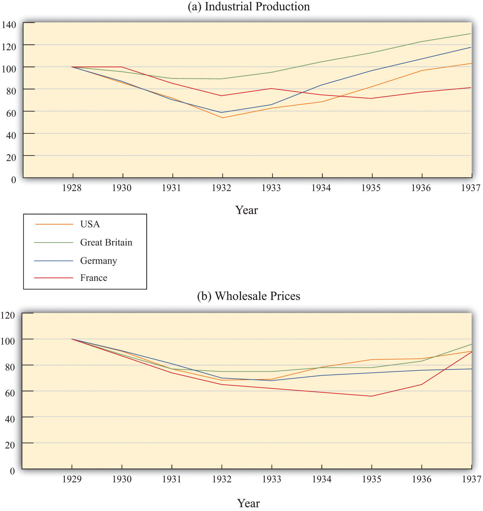
France, Germany, and Britain also experienced declines in output (a) and prices (b) during the Great Depression. The output data are data for industrial production (manufacturing in the case of the United States), and the price data are wholesale prices.
Source: International Monetary Fund, “World Economic Outlook: Crisis and Recovery,” April 2009, Box 3.1.1, http://www.imf.org/external/pubs/ft/weo/2009/01/c3/Box3_1_1.pdf.
Why this was the case remains one of the puzzles of the period. There were events at the time that had international dimensions, such as concerns about the future of the “gold standard” (which determined the exchange rates between countries) and various policies that disrupted international trade. Still, economists are unconvinced that such factors can explain why the Great Depression occurred in so many countries. Three-fourths of a century later, we still do not have a complete understanding of the Great Depression and are still unsure exactly why it happened. From one perspective this is frustrating, but from another it is exciting: the Great Depression maintains an air of mystery.
Toolkit: Section 31.20 "Foreign Exchange Market"
You can review the meaning and definition of the exchange rate in the toolkit.
The Puzzle of the Great Depression
Try to imagine yourself in the United States or Europe in the early 1930s. You are witnessing immense human misery amid a near meltdown of the economy. Friends and family are losing their jobs and have bleak prospects for new employment. Stores that you had shopped in all your life suddenly go out of business. The bank holding your money has disappeared, taking your savings with it. The government provides no insurance for unemployment, and there is no system of social security to provide support for your elderly relatives.
Economists and government officials at that time were bewildered. The experience in the United States and other countries was difficult to understand. According to the economic theories of the day, it simply was not possible. Policymakers had no idea how to bring about economic recovery. Yet, as you might imagine, there was considerable pressure for the government to do something about the problem. The questions that vexed the policymakers of the day—questions such as “What is happening?” and “What can the government do to help?”—are at the heart of this chapter.
Economists make sense of events like the Great Depression by first accumulating facts and then using frameworks to interpret those facts. We have a considerable advantage relative to economists and politicians at the time. We have the benefit of hindsight: the data we looked at in the previous subsection were not known to the economists of that era. And economic theory has evolved over the last seven decades, giving us better frameworks for analyzing these data.
Earlier, we said there are two possible reasons why output decreased.
- There was a decrease in production due to a decrease in the available inputs into the aggregate production function. Since there was no massive decrease in the amount of physical capital or the size of the workforce, and people presumably did not suddenly lose all their human capital, this means that the culprit must have been a decrease in technology.
- There was a decrease in aggregate spending. Households chose to reduce their consumption, firms chose to reduce their investment, and governments chose to reduce their spending. As a consequence, firms scaled back their production.
We look at each of these candidate explanations in turn.
Toolkit: Section 31.26 "The Aggregate Production Function"
You can review the aggregate production function and the inputs that go into it in the toolkit.
Key Takeaways
- During the Great Depression in the United States from 1929 to 1933, real GDP decreased by over 25 percent, the unemployment rate reached 25 percent, and prices decreased by over 9 percent in both 1931 and 1932 and by nearly 25 percent over the entire period.
- The Great Depression remains a puzzle today. Both the source of this large economic downturn and why it lasted for so long remain active areas of research and debate within economics.
- One explanation of the Great Depression rests on a reduction in the ability of the economy to produce goods and services. The second leading explanation focuses on a reduction in the overall demand for goods and services in the economy.
Checking Your Understanding
- The notes in Table 22.1 "Major Macroeconomic Variables, 1920–39*" state that the base year for the price level is 2000, so the price index has a value of 100 in that year. Approximately how much would you expect to have paid in the year 2000 for something that cost $2 in the late 1920s?
- Using Table 22.1 "Major Macroeconomic Variables, 1920–39*", how can you see that the unemployment rate is countercyclical?