This is “Where Do Prices Come From?”, chapter 7 from the book Theory and Applications of Economics (v. 1.0). For details on it (including licensing), click here.
For more information on the source of this book, or why it is available for free, please see the project's home page. You can browse or download additional books there. To download a .zip file containing this book to use offline, simply click here.


Chapter 7 Where Do Prices Come From?
The Price of a Pill
If you walk down the aisles of a supermarket, you will see thousands of different goods for sale. Each one will have a price displayed, telling you how much money you must give up if you want the good in question. On the Internet, you can find out how much it would cost you to stay in a hotel in Lima, Peru, or how much you would have to pay to rent a four-wheel drive vehicle in Nairobi, Kenya. On your television every evening, you can see the price that you would have to pay to buy a share of Microsoft Corporation or other companies.
Prices don’t appear by magic. Every price posted in the supermarket or on the Internet is the result of a decision made by one or more individuals. In the future, you may find yourself trying to make exactly such a decision. Many students of economics have jobs in the marketing departments of firms or work for consulting companies that provide advice on what prices firms should charge. To learn about how managers make such decisions, we look at a real-life pricing decision.
In 2003, a major pharmaceutical company was evaluating the performance of one of its most important drugs—a medication for treating high blood pressure—in a Southeast Asian country. (For reasons of confidentiality, we do not reveal the name of the company or the country; other than simplifying the numbers slightly, the story is true.) Its product was known as one of the best in the market and was being sold for $0.50 per pill. The company had good market share and income in the country. There was one major competing drug in the market that was selling at a higher price and a few less important drugs.
In pharmaceutical companies, one individual often leads the team for each major drug that the company sells. In this company, the head of the product team—we will call her Ellie—was happy with the performance of the drug. Nonetheless, she wondered whether her company could make higher profits by setting a higher or lower price. In many countries, the prices of pharmaceutical products are heavily regulated. In this particular country, however, pharmaceutical companies were largely free to set whatever price they chose. Together with her team, therefore, Ellie decided to review the pricing strategy for her product. In this chapter, we therefore tackle the following question:
How should a firm set its price?
Road Map
Price-setting in retail markets typically takes the form of a take-it-or-leave-it offer. The seller posts a price, and prospective customers either buy or don’t buy at that price. The prices you encounter every day in a supermarket, a coffee shop, or a fast-food restaurant, for example, are all take-it-or-leave-it offers that the retailer makes to you and other customers.Chapter 6 "eBay and craigslist" has more discussion.
In this chapter, we put you in the place of a marketing manager who has been given the job of determining the price that a firm should charge for its product. We first discuss the goals of this manager: what is she trying to achieve? We then show what information she needs to make a good decision. Finally, we derive some principles that allow her to set the right price. The chapter is built around two ideas:This chapter and Chapter 6 "eBay and craigslist" are linked because they are both about mechanisms that allocate goods and services. In Chapter 6 "eBay and craigslist" we explain how eBay, craigslist, and newspapers are ways in which individuals exchange goods and services. In this chapter, we study how goods and services are allocated from firms to households. At the end of this chapter, we show that the supply-and-demand framework introduced in Chapter 6 "eBay and craigslist" is also a useful framework when the same product is produced by a large number of firms. In particular, we show that our ideas about pricing also allow us to understand the foundations of supply.
- The law of demand. Each firm faces a demand curve for its product. This demand curve obeys the law of demand: if a firm sets a higher price, it must be willing to sell a smaller quantity; if a firm wishes to sell a larger quantity, it must set a lower price.
- Profit accounting. Firms earn income from selling their goods and services, but they also incur costs from producing those goods and services. These costs include the costs of raw materials, the wages paid to the firm’s workers, and so on. The difference between a firm’s revenues and its costs is the firm’s profits.
The choice of price, via the demand curve, determines the amount of output a firm sells. The amount of output determines a firm’s revenues and costs. Together, revenues and costs determine the profits of a firm.
7.1 The Goal of a Firm
Learning Objective
- What is the goal of a firm?
Firms devote substantial resources to their decisions about pricing. Large firms often have individuals or even entire departments whose main job is to make pricing decisions. Consulting firms specialize in providing advice to firms about the prices that they should charge. Some companies, such as airlines, have dedicated software to help them make these decisions. It isn’t hard to understand why firms pay so much attention to the prices they charge. More than anything else, price determines the profits that a firm earns.
Economists are prone to talk about the decisions and objectives of a firm, and we often use the same shorthand. A firm, though, is just a legal creation—a collection of individuals who use some kind of technology. A firm takes labor, raw materials, and other inputs and turns them into products that people want to buy. Some of the people in a firm—the managers—decide how many workers it should hire, what prices it should set, and so on.
To understand pricing, we begin with the goal of a firm (that is, its managers). If a firm’s managers are doing their jobs well, they should be making decisions to serve the interests of the owners of that firm. The owners of a firm are its shareholders. If you buy a share in a firm, then you own a fraction (your share) of the firm, which gives you the right to a fraction of the firm’s earnings. Shareholders, for the most part, have one reason for buying and owning shares: to earn income. So the managers, if they are doing their jobs well, want a firm to make as much money as possible. We need to be careful, though. What matters is not the total amount of money received by a firm, but how much is available to be distributed to its owners. The owners of a firm hope to earn as high a return as possible on their shares.
Toolkit: Section 31.15 "Pricing with Market Power"
The money that is available for distribution to the shareholders of a firm is called a firm’s profits. A firm pays money for raw materials, energy, and other supplies, and it pays wages to its workers. These expenses are a firm’s costs of production. When it sells the product(s) it has produced, a firm earns revenues. Accountants analyze these revenues and costs in more detail, but in the end all the monies that flow in and out of a firm can be classified as either revenues or costs. Thus
profits = revenues − costs.Consider, then, a marketing manager who wants to set the best price for a product—such as Ellie choosing the price for her company’s blood pressure medication. She wants to find the price that will yield the most profits to her company. In an ideal world, a marketing manager might have access to a spreadsheet table, such as Figure 7.1 "A Spreadsheet That Would Make Pricing Decisions Easy", which displays a firm’s monthly profits for different possible prices that it might set. Then Ellie’s job would be easy: she would just have to look at the table, find the cell in column B with the highest number, and set the corresponding price. In this case, she would set a price of $15.
Figure 7.1 A Spreadsheet That Would Make Pricing Decisions Easy
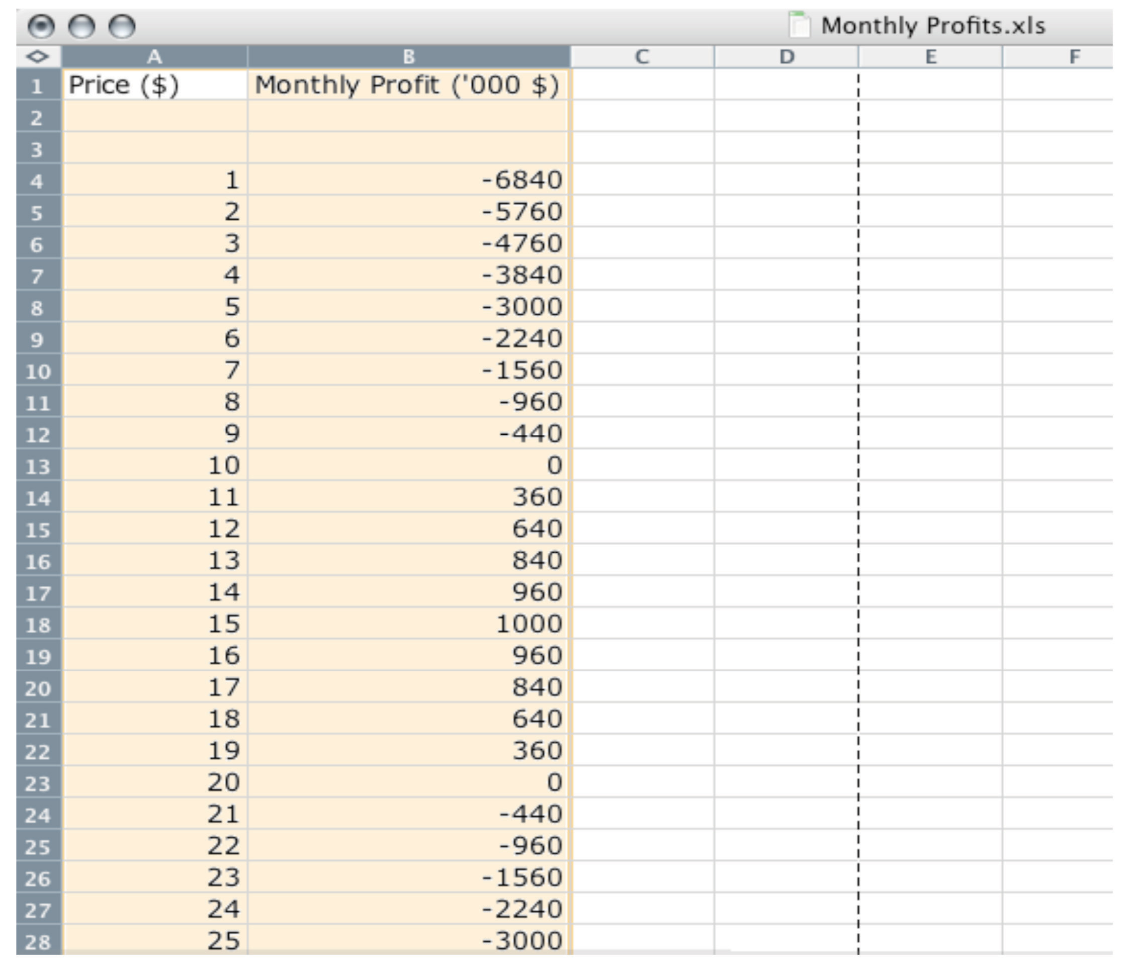
But the reality of business is different. It is very difficult and expensive—perhaps even impossible—to gather information such as that in Figure 7.1 "A Spreadsheet That Would Make Pricing Decisions Easy". You might imagine that a firm could experiment, trying different prices and seeing what profitsRevenues minus costs. it earned. Unfortunately, this would be very costly because most of the time a firm would earn much lower profits than it could. Experimenting might even generate losses. For example, suppose that, one September, Ellie chose to try a price of $2 per pill. The firm would lose nearly $6 million—the equivalent of about six months’ profits even at the very best price. Ellie would rapidly find herself looking for another job.
It is clear that trial and error—choosing different prices at random and seeing how much profit you get—could lead to costly mistakes, and there is no guarantee that you would ever find the best price. By adding some structure to a trial-and-error process, though, there is a simple strategy for finding the best price: begin by slightly raising the firm’s price. If profits increase, then you are on the right track. Keep raising the price, little by little, until profits stop increasing. On the other hand, if profits decrease when you raise the price, then you should try lowering the price instead. If profits increase, then keep lowering the price little by little.
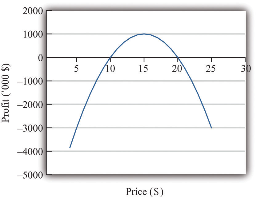
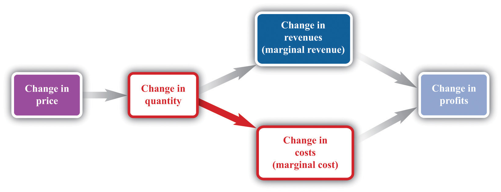
Figure 7.2 "A Change in Price Leads to a Change in Profits" shows how a change in price translates into a change in profits. A change in a firm’s price leads to a change in the quantity demanded. As a result, the revenuesWhat a firm receives for selling its output, which is equal to the price received per unit sold times the number of units sold. and costsThe payments a firm makes for its inputs, such as wages for its workers. of a firm change, as do its profits. Figure 7.3 "The Profits of a Firm" shows the profits a firm will earn at different prices. Our pricing strategy simply says the following. You are trying to get to the highest point of the profit hill in Figure 7.3 "The Profits of a Firm", and you will get there eventually if you always walk uphill. At the very top of the hill, the change in profits is zero.
Figure 7.2 A Change in Price Leads to a Change in Profits
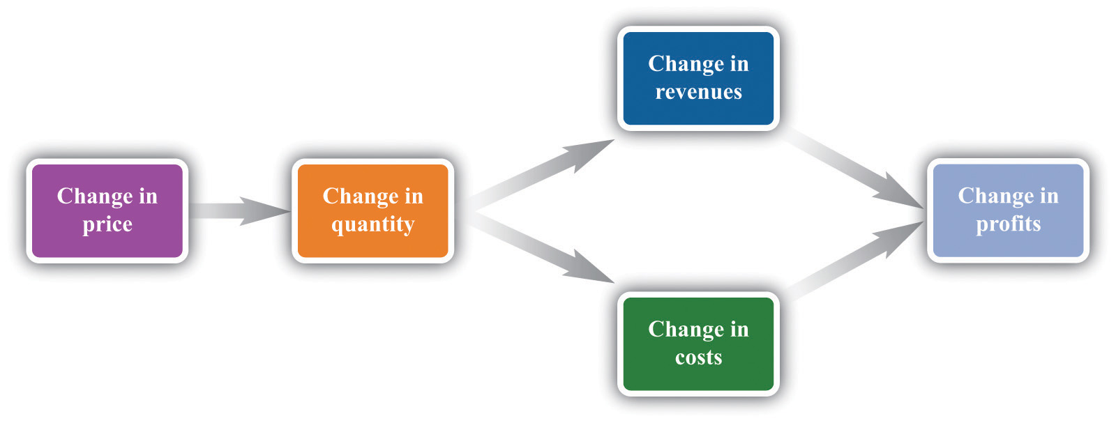
If a firm changes its price, then there will be a change in demand. This then leads to changes in revenues and costs, which changes in the profits of a firm.
Figure 7.3 The Profits of a Firm
We could end the chapter right here. But we want to dig deeper and uncover some principles that tell us more about how pricing works. Then we can learn what information Ellie and other managers like her need to make better pricing decisions—and how they can make these decisions effectively. Our starting point is our earlier observation that
profits = revenues − costs.Key Takeaway
- The objective of a firm is to maximize its profits, defined as revenues minus costs.
Checking Your Understanding
- If the manager of a firm chose a price to maximize sales, what would that price be? What would profits be at that price?
- Explain in words why the profit function has the shape shown in Figure 7.3 "The Profits of a Firm".
7.2 The Revenues of a Firm
Learning Objectives
- What is the demand curve faced by a firm?
- What is the elasticity of demand? How is it calculated?
- What is marginal revenue?
A firm’s revenues are the money that it earns from selling its product. Revenues equal the number of units that a firm sells times the price at which it sells each unit:
revenues = price × quantity.For example, think about a music store selling CDs. Suppose that the firm sells 25,000 CDs in a month at $15 each. Then its total monthly revenues are as follows:
revenues = 15 × 25,000 = $375,000.There are two ways in which firms can obtain higher revenues: sell more products or sell at a higher price. So if a firm wants to make a lot of revenue, it should sell a lot of its product at a high price. Then again, you probably do not need to study economics to figure that out. The problem for a manager is that her ability to sell a product is limited by what the market will bear. Typically, we expect that if she sets a higher price, she will not be able to sell as much of the product:
Equivalently, if she wants to sell a larger quantity of product, she will need to drop the price:
This is the law of demand in operation (Figure 7.4 "A Change in the Price Leads to a Change in Demand").
Figure 7.4 A Change in the Price Leads to a Change in Demand
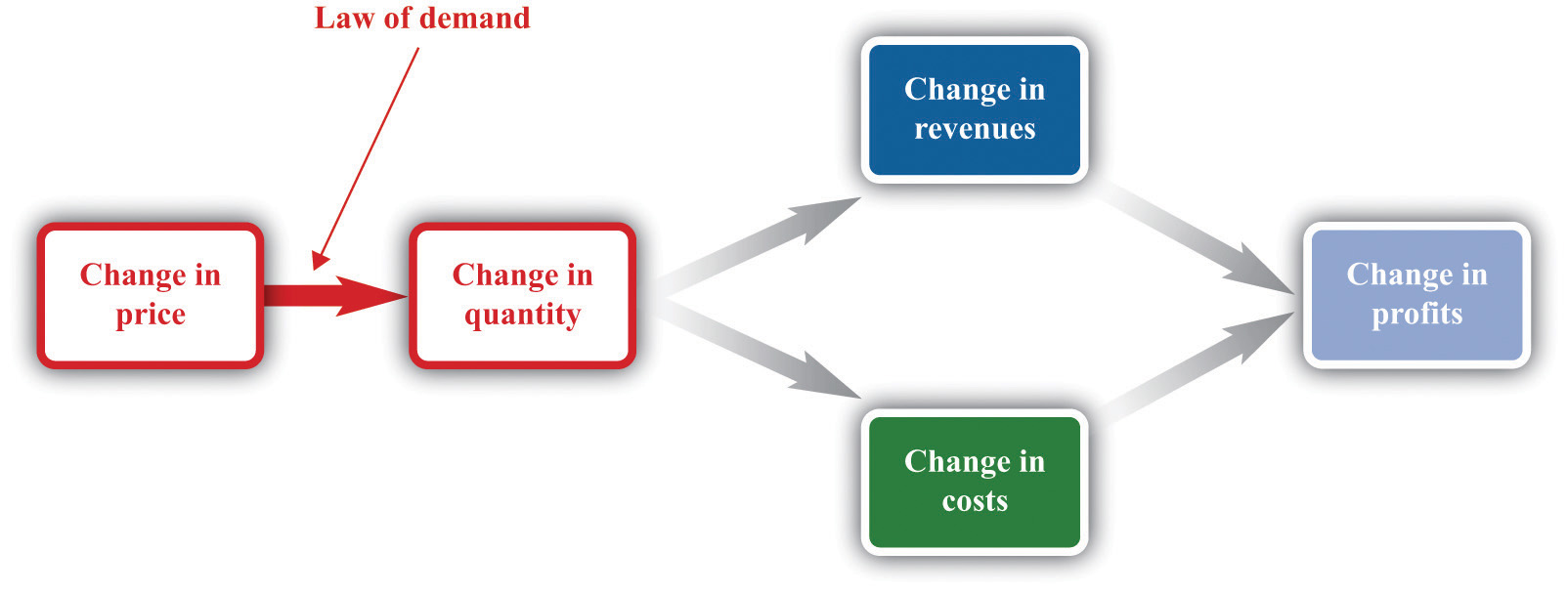
An increase in price leads to a decrease in demand. A decrease in price leads to an increase in demand.
The Demand Curve Facing a Firm
There will typically be more than one firm that serves a market. This means that the overall demand for a product is divided among the different firms in the market. We have said nothing yet about the kind of “market structure” in which a firm is operating—for example, does it have a lot of competitors or only a few competitors? Without delving into details, we cannot know exactly how the market demand curve will be divided among the firms in the market. Fortunately, we can put this problem aside—at least for this chapter.We look at market structure in Chapter 15 "Busting Up Monopolies". For the moment, it is enough just to know that each firm faces a demand curve for its own product.
When the price of a product increases, individual customers are less likely to think it is good value and are more likely to spend their income on other things instead. As a result—for almost all products—a higher price leads to lower sales.
Toolkit: Section 31.15 "Pricing with Market Power"
The demand curve facing a firm tells us the price that a firm can expect to receive for any given amount of output that it brings to market or the amount it can expect to sell for any price that it chooses to set. It represents the market opportunities of the firm.
An example of such a demand curve is
quantity demanded = 100 − (5 × price).Table 7.1 "Example of the Demand Curve Faced by a Firm" calculates the quantity associated with different prices. For example, with this demand curve, if a manager sets the price at $10, the firm will sell 50 units because 100 − (5 × 10) = 50. If a manager sets the price at $16, the firm will sell only 20 units: 100 − (5 × 16) = 20. For every $1 increase in the price, output decreases by 5 units. (We have chosen a demand curve with numbers that are easy to work with. If you think that this makes the numbers unrealistically small, think of the quantity as being measured in, say, thousands of units, so a quantity of 3 in this equation means that the firm is selling 3,000 units. Our analysis would be unchanged.)
Table 7.1 Example of the Demand Curve Faced by a Firm
| Price ($) | Quantity |
|---|---|
| 0 | 100 |
| 2 | 90 |
| 4 | 80 |
| 6 | 70 |
| 8 | 60 |
| 10 | 50 |
| 12 | 40 |
| 14 | 30 |
| 16 | 20 |
| 18 | 10 |
| 20 | 0 |
Equivalently, we could think about a manager choosing the quantity that the firm should produce, in which case she would have to accept the price implied by the demand curve. To write the demand curve this way, first divide both sides of the equation by 5 to obtain
Now add “price” to each side and subtract “” from each side:
For example, if the manager wants to sell 70 units, she will need a price of $6 (because 20 − 70/5 = 6). For every unit increase in quantity, the price decreases by 20 cents.
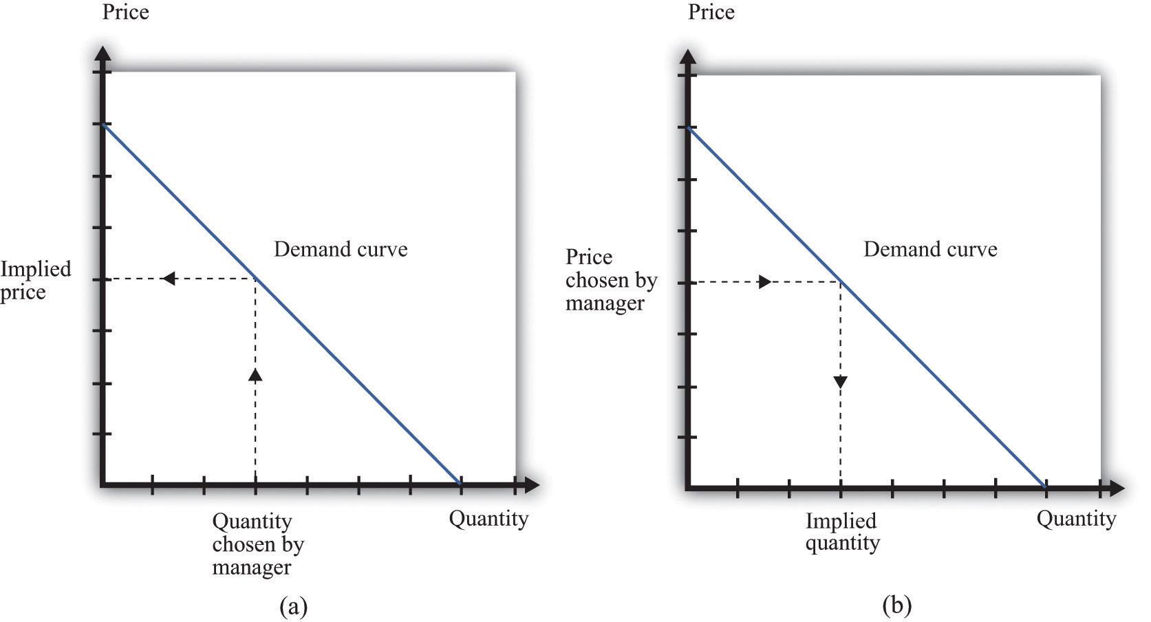
Either way of looking at the demand curve is perfectly correct. Figure 7.5 "Two Views of the Demand Curve" shows the demand curve in these two ways. Look carefully at the two parts of this figure and convince yourself that they are really the same—all we have done is switch the axes.
Figure 7.5 Two Views of the Demand Curve
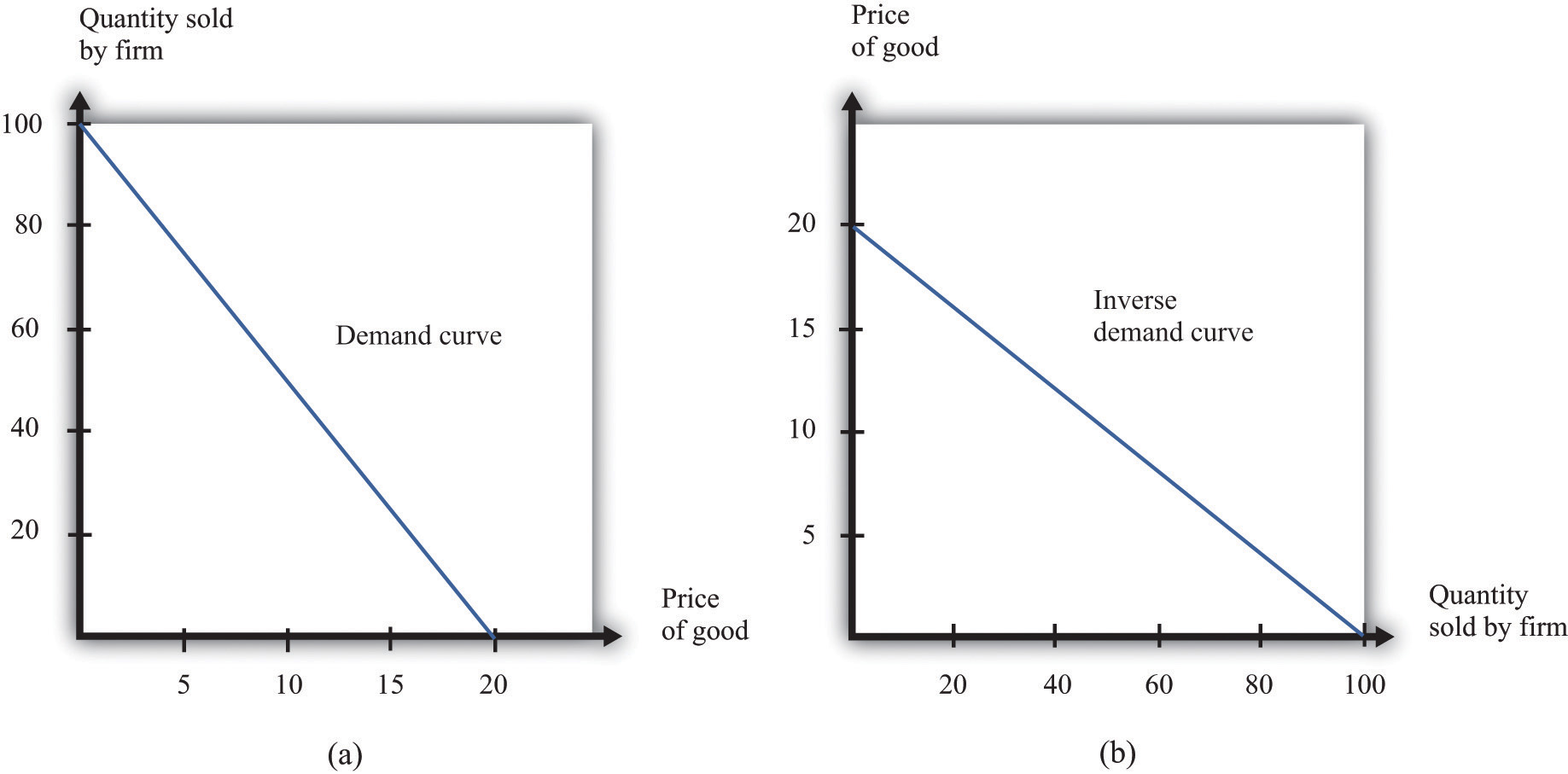
There are two ways that we can draw a demand curve, both of which are perfectly correct. (a) The demand curve has price on the horizontal axis and quantity demanded on the vertical axis (b). The demand curve has price on the vertical axis, which is how we normally draw the demand curve in economics.
The firm faces a trade-off: it can set a high price, such as $18, but it will be able to sell only a relatively small quantity (10). Alternatively, the firm can sell a large quantity (for example, 80), but only if it is willing to accept a low price ($4). The hard choice embodied in the demand curve is perhaps the most fundamental trade-off in the world of business. Of course, if the firm sets its price too high, it won’t sell anything at all. The choke priceThe price above which no units of the good will be sold. is the price above which no units of the good will be sold. In our example, the choke price is $20; look at the vertical axis in part (b) of Figure 7.5 "Two Views of the Demand Curve".A small mathematical technicality: the equation for the demand curve applies only if both the price and the quantity are nonnegative. At any price greater than the choke price, the quantity demanded is zero, so the demand curve runs along the vertical axis. A negative price would mean a firm was paying consumers to take the product away.
Every firm in the economy faces some kind of demand curve. Knowing the demand for your product is one of the most fundamental necessities of successful business. We therefore turn next to the problem Ellie learned about the demand curve for her company’s drug.
The Elasticity of Demand: How Price Sensitive Are Consumers?
Marketing managers understand the law of demand. They know that if they set a higher price, they can expect to sell less output. But this is not enough information for good decision making. Managers need to know whether their customers’ demand is very sensitive or relatively insensitive to changes in the price. Put differently, they need to know if the demand curve is steep (a change in price will lead to a small change in output) or flat (a change in price will lead to a big change in output). We measure this sensitivity by the own-price elasticity of demandThe percentage change in quantity demanded of a good divided by the percentage change in the price of that good..
Toolkit: Section 31.2 "Elasticity"
The own-price elasticity of demand (often simply called the elasticity of demand) measures the response of quantity demanded of a good to a change in the price of that good. Formally, it is the percentage change in the quantity demanded divided by the percentage change in the price:
When price increases (the change in the price is positive), quantity decreases (the change in the quantity is negative). The price elasticity of demand is a negative number. It is easy to get confused with negative numbers, so we instead use
which is always a positive number.
- If −(elasticity of demand) is a large number, then quantity demanded is sensitive to price: increases in price lead to big decreases in demand.
- If −(elasticity of demand) is a small number, then quantity demanded is insensitive to price: increases in price lead to small decreases in demand.
Throughout the remainder of this chapter, you will often see −(elasticity of demand). Just remember that this expression always refers to a positive number.
Calculating the Elasticity of Demand: An Example
Go back to our earlier example:
quantity demanded = 100 − 5 × price.Suppose a firm sets a price of $15 and sells 25 units. What is the elasticity of demand if we think of a change in price from $15 to $14.80? In this case, the change in the price is −0.2, and the change in the quantity is 1. Thus we calculate the elasticity of demand as follows:
- The percentage change in the quantity is (4 percent).
- The percentage change in the price is (approximately −1.3 percent).
- −(elasticity of demand) is
The interpretation of this elasticity is as follows: when price decreases by 1 percent, quantity demanded increases by 3 percent. This is illustrated in Figure 7.6 "The Elasticity of Demand".
Figure 7.6 The Elasticity of Demand
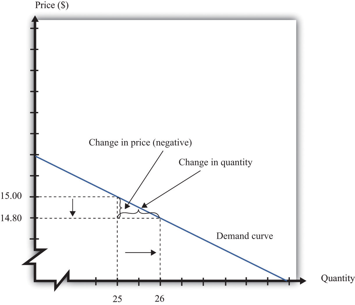
When the price is decreased from $15.00 to $14.80, sales increase from 25 to 26. The percentage change in price is −1.3 percent. The percentage change in the quantity sold is 4. So −(elasticity of demand) is 3.
One very useful feature of the elasticity of demand is that it does not change when the number of units changes. Suppose that instead of measuring prices in dollars, we measure them in cents. In that case our demand curve becomes
quantity demanded = 100 − 500 × price.Make sure you understand that this is exactly the same demand curve as before. Here the slope of the demand curve is −500 instead of −5. Looking back at the formula for elasticity, you see that the change in the price is 100 times greater, but the price itself is 100 times greater as well. The percentage change is unaffected, as is elasticity.
Market Power
The elasticity of demand is very useful because it is a measure of the market powerThe extent to which a firm produces a product that consumers want very much and for which few substitutes are available. that a firm possesses. In some cases, some firms produce a good that consumers want very much—a good in which few substitutes are available. For example, De Beers controls much of the world’s market for diamonds, and other firms are not easily able to provide substitutes. Thus the demand for De Beers’ diamonds tends to be insensitive to price. We say that De Beers has a lot of market power. By contrast, a fast-food restaurant in a mall food court possesses very little market power: if the fast-food Chinese restaurant were to try to charge significantly higher prices, most of its potential customers would choose to go to the other Chinese restaurant down the aisle or even to eat sushi, pizza, or burritos instead.
Ellie’s company had significant market power. There were a relatively small number of drugs available in the country to treat high blood pressure, and not all drugs were identical in terms of their efficacy and side effects. Some doctors were loyal to her product and would almost always prescribe it. Some doctors were not very well informed about the price because doctors don’t pay for the medication. For all these reasons, Ellie had reason to suspect that the demand for her drug was not very sensitive to price.
The Elasticity of Demand for a Linear Demand Curve
The elasticity of demand is generally different at different points on the demand curve. In other words, the market power of a firm is not constant: it depends on the price that a firm has chosen to set. To illustrate, remember that we found −(elasticity of demand) = 3 for our demand curve when the price is $15. Suppose we calculate the elasticity for this same demand curve at $4. Thus imagine that that we are originally at the point where the price is $4 and sales are 80 units and then suppose we again decrease the price by 20 cents. Sales will increase by 1 unit:
- The percentage change in the quantity is (1.25 percent).
- The percentage change in the price is (5 percent).
- −(elasticity of demand) is
The elasticity of demand is different because we are at a different point on the demand curve.
When −(elasticity of demand) increases, we say that demand is becoming more elastic. When −(elasticity of demand) decreases, we say that demand is becoming less elastic. As we move down a linear demand curve, −(elasticity of demand) becomes smaller, as shown in Figure 7.7 "The Elasticity of Demand When the Demand Curve Is Linear".
Figure 7.7 The Elasticity of Demand When the Demand Curve Is Linear
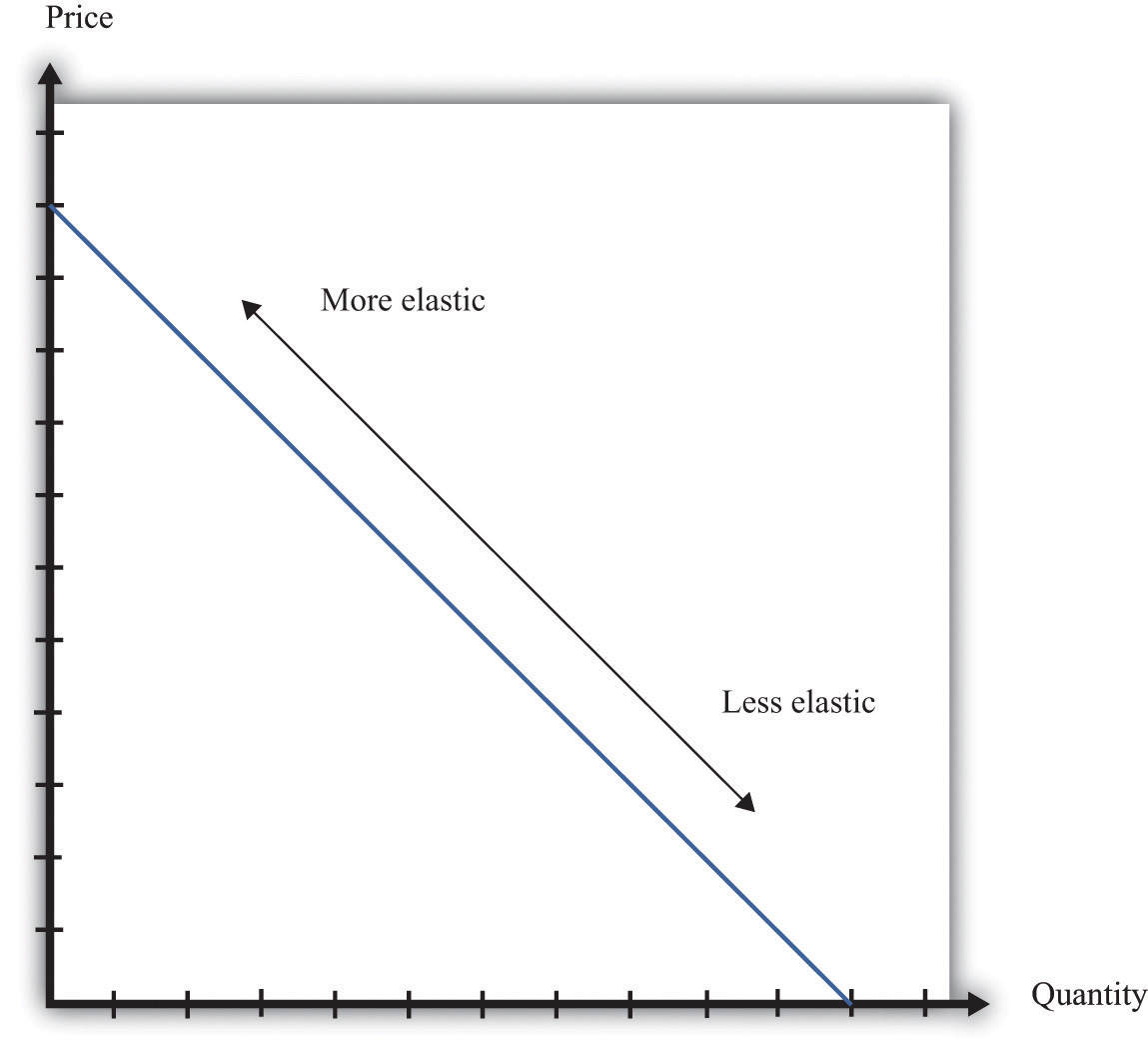
The elasticity of demand is generally different at different points on a demand curve. In the case of a linear demand curve, −(elasticity of demand) becomes smaller as we move down the demand curve.
Measuring the Elasticity of Demand
To evaluate the effects of her decisions on revenues, Ellie needs to know about the demand curve facing her firm. In particular, she needs to know whether the quantity demanded by buyers is very sensitive to the price that she sets. We now know that the elasticity of demand is a useful measure of this sensitivity. How can managers such as Ellie gather information on the elasticity of demand?
At an informal level, people working in marketing and sales are likely to have some idea of whether their customers are very price sensitive. Marketing and sales personnel—if they are any good at their jobs—spend time talking to actual and potential customers and should have some idea of how much these customers care about prices. Similarly, these employees should have a good sense of the overall market and the other factors that might affect customers’ choices. For example, they will usually know whether there are other firms in the market offering similar products, and, if so, what prices these firms are charging. Such knowledge is much better than nothing, but it does not provide very concrete evidence on the demand curve or the elasticity of demand.
A firm may be able to make use of existing sales data to develop a more concrete measure of the elasticity of demand. For example, a firm might have past sales data that show how much they managed to sell at different prices, or a firm might have sales data from different cities where different prices were charged. Suppose a pricing manager discovers data for prices and quantities like those in part (a) of Figure 7.8 "Finding the Demand Curve". Here, each dot marks an observation—for example, we can see that in one case, when the price was $100, the quantity demanded was 28.
Figure 7.8 Finding the Demand Curve
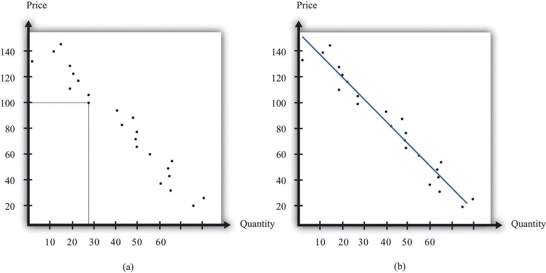
(a) This is an example of data that a manager might have obtained for prices and quantities. (b) A line is fit to the data that represents a best guess at the underlying demand curve facing a firm.
The straight-line demand curves that appear in this and other books are a convenient fiction of economists and textbook writers, but no one has actually seen one in captivity. In the real world of business, demand curves—if they are available at all—are only a best guess from a collection of data. Economists and statisticians have developed statistical techniques for these guesses. The underlying idea of these techniques is that they fit a line to the data. (The exact details do not concern us here; you can learn about them in more advanced courses in economics and statistics.) Part (b) of Figure 7.8 "Finding the Demand Curve" shows an example. It represents our best prediction, based on available data, of how much people will buy at different prices.
If a firm does not have access to reliable existing data, a third option is for it to generate its own data. For example, suppose a retailer wanted to know how sensitive customer demand for milk is to changes in the price of milk. It could try setting a different price every week and observe its sales. It could then plot them in a diagram like Figure 7.8 "Finding the Demand Curve" and use techniques like those we just discussed to fit a line. In effect, the store could conduct its own experiment to find out what its demand curve looks like. For a firm that sells over the Internet, this kind of experiment is particularly attractive because it can randomly offer different prices to people coming to its website.
Finally, firms can conduct market research either on their own or by hiring a professional market research firm. Market researchers use questionnaires and surveys to try to discover the likely purchasing behavior of consumers. The simplest questionnaire might ask, “How much would you be willing to pay for product x?” Market researchers have found such questions are not very useful because consumers do not answer them very honestly. As a result, research firms use more subtle questions and other more complicated techniques to uncover consumers’ willingness to pay for goods and services.
Ellie decided that she should conduct market research to help with the pricing decision. She hired a market research firm to ask doctors about how they currently prescribed different high blood pressure medications. Specifically, the doctors were asked what percentage of their prescriptions went to each of the drugs on the market. Then they were asked the effect of different prices on those percentages. Based on this research, the market research firm found that a good description of the demand curve was as follows:
quantity demanded = 252 − 300 × price.Remember that the drug was currently being sold for $0.50 a pill, so
quantity demanded = 252 − 300 × 0.5 = 102.The demand curve also told Ellie that if she increased the price by 10 percent to $0.55, the quantity demanded would decrease to 87 (252 − 300 × 0.55 = 87). Therefore, the percentage change in quantity is From this, the market research firm discovered that the elasticity of demand at the current price was
How Do Revenues Depend on Price?
The next step is to understand how to use the demand curve when setting prices. The elasticity of demand describes how quantity demanded depends on price, but what a manager really wants to know is how revenues are affected by price. Revenues equal price times quantity, so we know immediately that a firm earns $0 if the price is $0. (It doesn’t matter how much you give away, you still get no money.) We also know that, at the choke price, the quantity demanded is 0 units, so its revenues are likewise $0. (If you sell 0 units, it doesn’t matter how high a price you sell them for.) At prices between $0 and the choke price, however, the firm sells a positive amount at a positive price, thus earning positive revenues. Figure 7.9 "Revenues" is a graphical representation of the revenues of a firm. Revenues equal price times quantity, which is the area of the rectangle under the demand curve. For example, at $14 and 30 units, revenues are $420.
Figure 7.9 Revenues
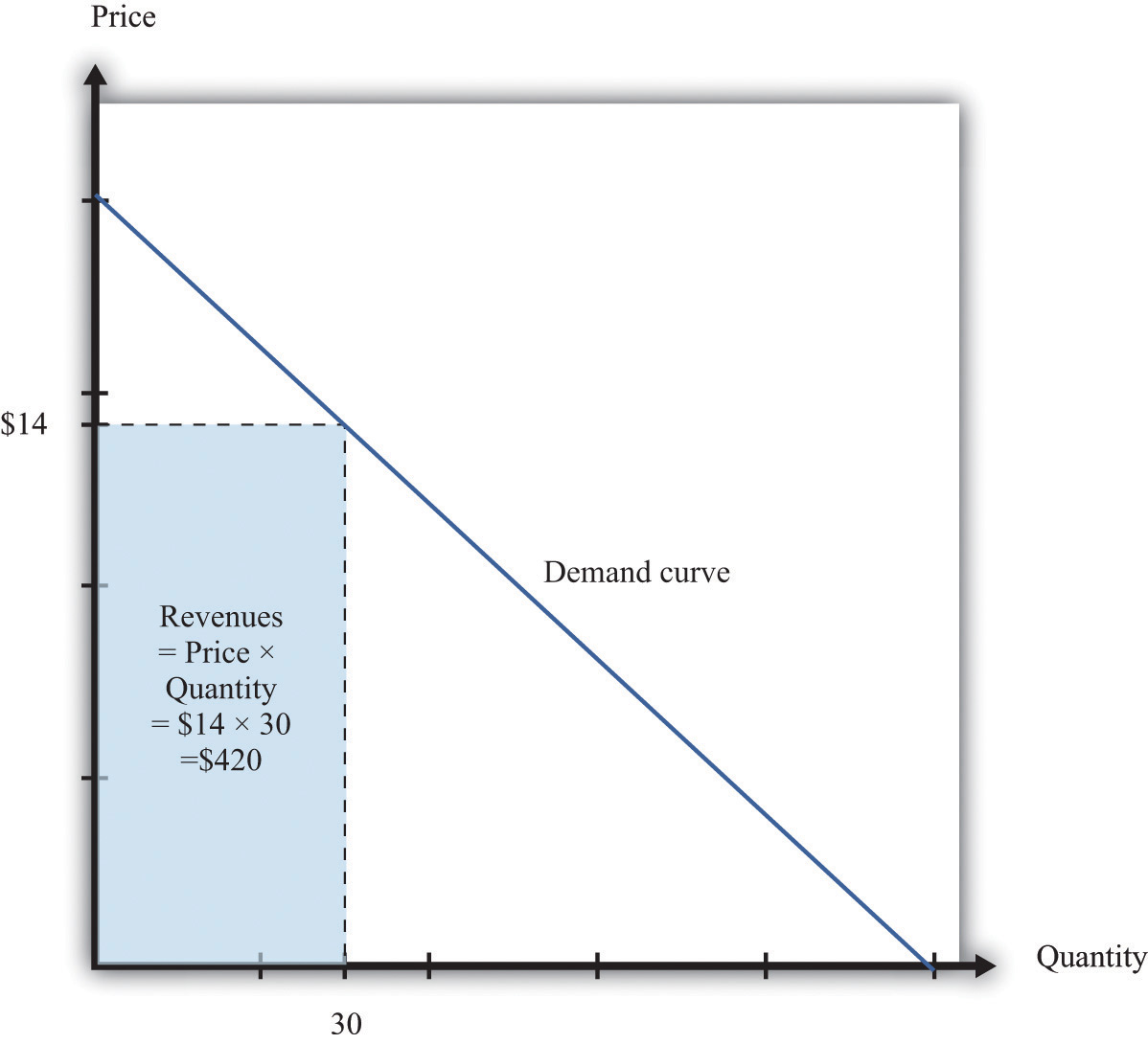
The revenues of a firm are equal to the area of the rectangle under the demand curve.
We can use the information in Table 7.1 "Example of the Demand Curve Faced by a Firm" to calculate the revenues of a firm at different quantities and prices (this is easy to do with a spreadsheet). Table 7.2 "Calculating Revenues" shows that if we start at a price of zero and increase the price, the firm’s revenues also increase. Above a certain point, however (in this example, $10), revenues start to decrease again.
Table 7.2 Calculating Revenues
| Price($) | Quantity | Revenues ($) |
|---|---|---|
| 0 | 100 | 0 |
| 2 | 90 | 180 |
| 4 | 80 | 320 |
| 6 | 70 | 420 |
| 8 | 60 | 480 |
| 10 | 50 | 500 |
| 12 | 40 | 480 |
| 14 | 30 | 420 |
| 16 | 20 | 320 |
| 18 | 10 | 180 |
| 20 | 0 | 0 |
Marginal Revenue
Earlier we suggested that a good strategy for pricing is to experiment with small changes in price. So how do small changes in price affect the revenue of a firm? Suppose, for example, that a firm has set the price at $15 and sells 25 units, but the manager contemplates decreasing the price to $14.80. We can see the effect that this has on the firm’s revenues in Figure 7.10 "Revenues Gained and Lost".
Figure 7.10 Revenues Gained and Lost
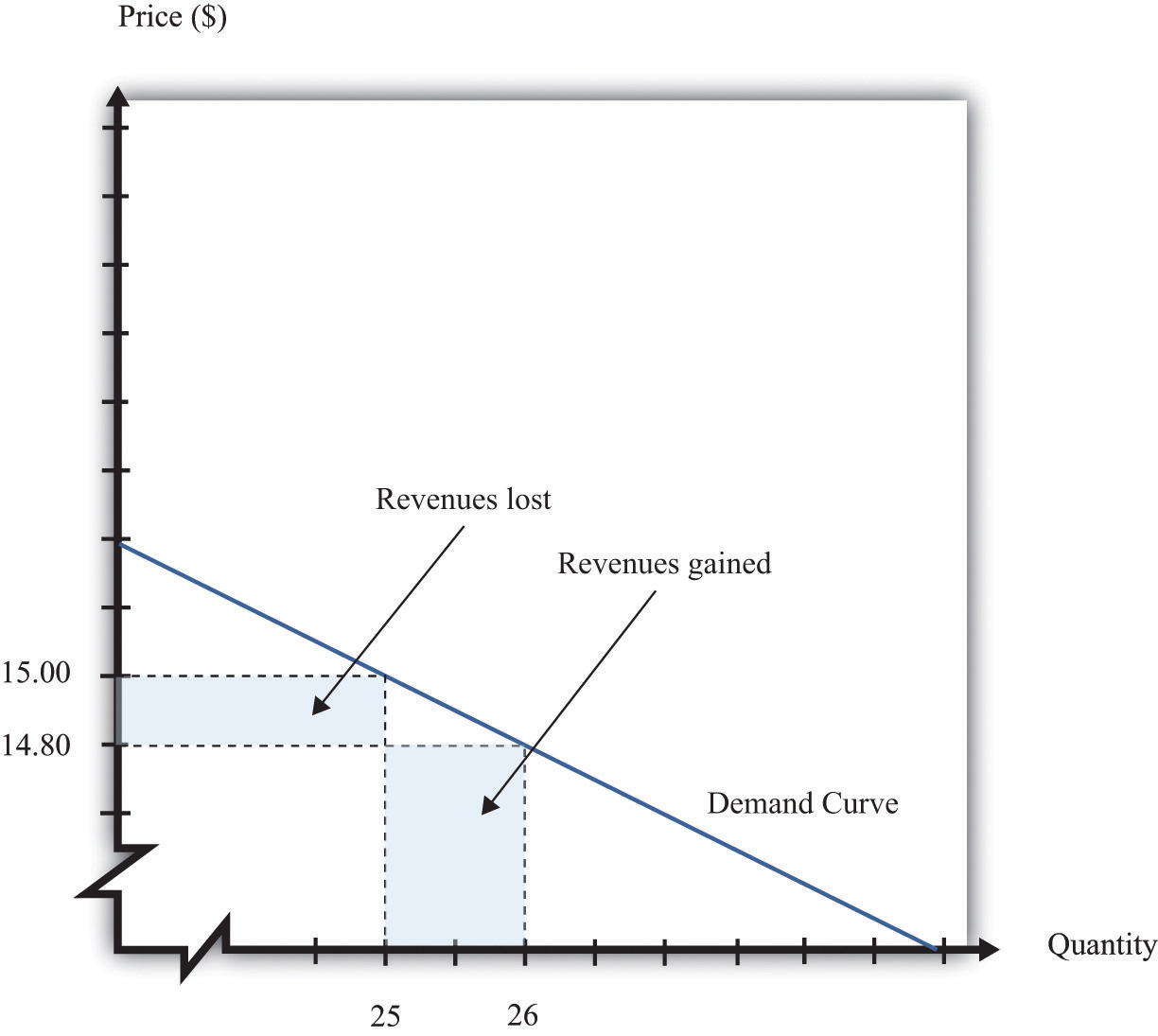
If a firm cuts its price, it sells more of its product, which increases revenues, but sells each unit at a lower price, which decreases revenues.
The firm will lose 20 cents on each unit it sells, so it will lose $5 in revenue. This is shown in the figure as the rectangle labeled “revenues lost.” But the firm will sell more units: from the demand curve, we know that when the firm decreases its price by $0.20, it sells another unit. That means that the firm gains $14.80, as shown in the shaded area labeled “revenues gained.” The overall change in the firm’s revenues is equal to $14.80 − $5.00 = $9.80. Decreasing the price from $15.00 to $14.80 will increase its revenues by $9.80.
Look carefully at Figure 7.10 "Revenues Gained and Lost" and make sure you understand the experiment. We presume throughout this chapter that a firm must sell every unit at the same price. When we talk about moving from $15.00 to $14.80, we are not supposing that a firm sells 25 units for $15 and then drops its price to $14.80 to sell the additional unit. We are saying that the manager is choosing between selling 25 units for $15.00 or 26 units for $14.80.
Figure 7.11 Calculating the Change in Revenues
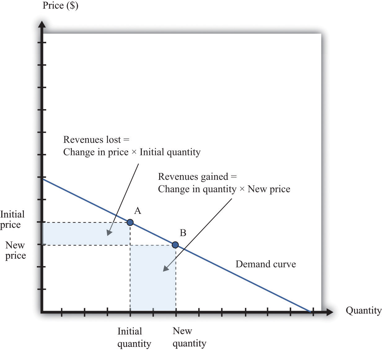
If a manager has an idea about how much quantity demanded will decrease for a given increase in price, she can calculate the likely effect on revenues.
Figure 7.11 "Calculating the Change in Revenues" explains this idea more generally. Suppose a firm is originally at point A on the demand curve. Now imagine that a manager decreases the price. At the new, lower price, the firm sells a new, higher quantity (point B). The change in the quantity is the new quantity minus the initial quantity. The change in the price is the new price minus the initial price (remember that this is a negative number). The change in the firm’s revenues is given by
change in revenues = (change in quantity × new price) + (change in price × initial quantity).The first term is positive: it is the extra revenue from selling the extra output. The second term is negative: it is the revenue lost because the price has been decreased. Together these give the effect of a change in price on revenues, which we call a firm’s marginal revenueThe extra revenue from selling an additional unit of output, which is equal to the change in revenue divided by the change in sales..
Toolkit: Section 31.15 "Pricing with Market Power"
Marginal revenue is the change in revenue associated with a change in quantity of output sold:
We can write this asFor the derivation of this expression, see the toolkit.
Marginal Revenue and the Elasticity of Demand
Given the definitions of marginal revenue and the elasticity of demand, we can write
It may look odd to write this expression with two minus signs. We do this because it is easier to deal with the positive number: −(elasticity of demand). We see three things:
- Marginal revenue is always less than the price. Mathematically, Suppose a firm sells an extra unit. If the price stays the same, then the extra revenue would just equal the price. But the price does not stay the same: it decreases, meaning the firm gets less for every unit that it sells.
- Marginal revenue can be negative. If –(elasticity of demand) < 1, then and When marginal revenue is negative, increased production results in lower revenues for a firm. The firm sells more output but loses more from the lower price than it gains from the higher sales.
- The gap between marginal revenue and price depends on the elasticity of demand. When demand is more elastic, meaning −(elasticity of demand) is a bigger number, the gap between marginal revenue and price becomes smaller.
These three ideas are illustrated in Figure 7.12 "Marginal Revenue and Demand". The demand curve shows us the price at any given quantity. The marginal revenue curve lies below the demand curve because of our first observation: at any quantity, marginal revenue is less than price.When a demand curve is a straight line, the marginal revenue curve is also a straight line with the same intercept, but it is twice as steep. The marginal revenue curve intersects the horizontal axis at 50 units: when output is less than 50 units, marginal revenue is positive; when output exceeds 50, marginal revenue is negative. We explained earlier that a linear demand curve becomes more inelastic as you move down it. When the demand curve goes from being relatively elastic to relatively inelastic, marginal revenue goes from being positive to being negative.
Figure 7.12 Marginal Revenue and Demand
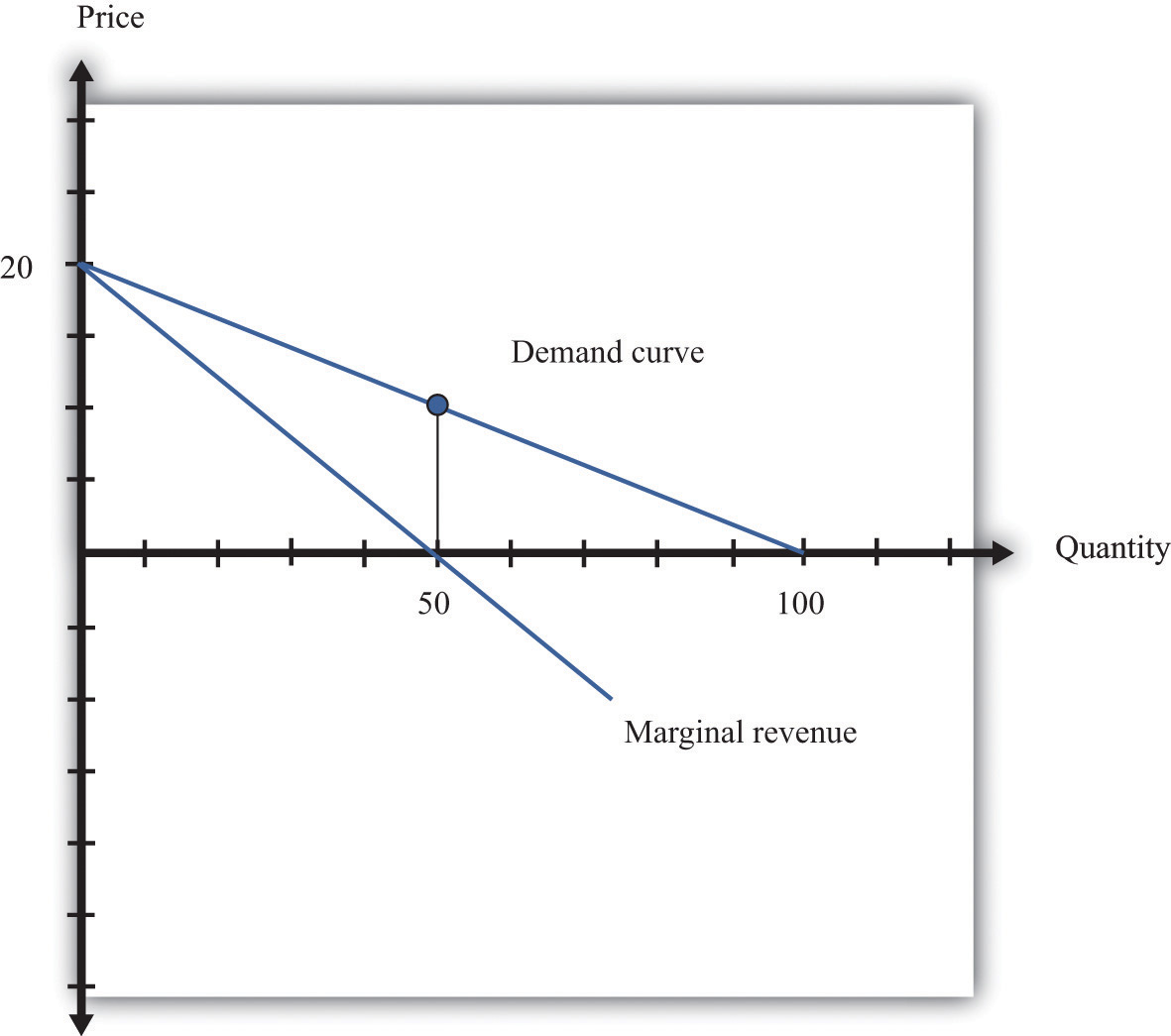
The marginal revenue curve lies below the demand curve because at any quantity, marginal revenue is less than price.
Earlier, we showed that when a firm sets the price at $15, −(elasticity of demand) = 3. Thus we can calculate marginal revenue at this price:
What does this mean? Starting at $15, it means that if a firm decreases its price—and hence increase its output—by a small amount, there would be an increase in the firm’s revenues.
When revenues are at their maximum, marginal revenue is zero. We can confirm this by calculating the elasticity of demand at $10. Consider a 10 percent increase in price, so the price increases to $11. At $10, sales equal 50 units. At $11, sales equal 45 units. In other words, sales decrease by 5 units, so the decrease in sales is 10 percent. It follows that
Plugging this into our expression for marginal revenue, we confirm that
At $10, a small change in price leads to no change in revenue. The benefit from selling extra output is exactly offset by the loss from charging a lower price.
Figure 7.13 Marginal Revenue and the Elasticity of Demand
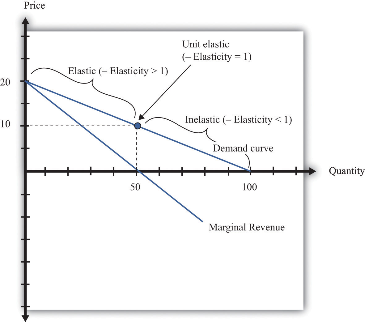
The demand curve can be divided into two parts: at low quantities and high prices, marginal revenue is positive and the demand curve is elastic; at high quantities and low prices, marginal revenue is negative and the demand curve is inelastic.
We can thus divide the demand curve into two parts, as in Figure 7.13 "Marginal Revenue and the Elasticity of Demand". At low quantities and high prices, a firm can increase its revenues by moving down the demand curve—to lower prices and higher output. Marginal revenue is positive. In this region, −(elasticity of demand) is a relatively large number (specifically, it is between 1 and infinity) and we say that the demand curve is relatively elastic. Conversely, at high quantities and low prices, a decrease in price will decrease a firm’s revenues. Marginal revenue is negative. In this region, −(elasticity of demand) is between 0 and 1, and we say that the demand curve is inelastic. Table 7.3 represents this schematically.
Table 7.3
| −(Elasticity of Demand) | Demand | Marginal Revenue | Effect of a Small Price Decrease |
|---|---|---|---|
| • > –(elasticity of demand) > 1 | Relatively elastic | Positive | Increase revenues |
| −(elasticity of demand) = 1 | Unit elastic | Zero | Have no effect on revenues |
| 1 > –(elasticity of demand) > 0 | Relatively inelastic | Negative | Decrease revenues |
Maximizing Revenues
The market research company advising Ellie made a presentation to her team. The company told them that if they increased their price, they could expect to see a decrease in revenue. At their current price, in other words, marginal revenue was positive. If Ellie’s team wanted to maximize revenue, they would need to recommend a reduction in price: down to the point where marginal revenue is $0—equivalently, where −(elasticity of demand) = 1.
Some members of Ellie’s team therefore argued that they should try to decrease the price of the product so that they could increase their market share and earn more revenues from the sale of the drug. Ellie reminded them, though, that their goal wasn’t to have as much revenue as possible. It was to have as large a profit as possible. Before they could decide what to do about price, they needed to learn more about the costs of producing the drug.
Key Takeaways
- The demand curve tells a firm how much output it can sell at different prices.
- The elasticity of demand is the percentage change in quantity divided by the percentage change in the price.
- Marginal revenue is the change in total revenue from a change in the quantity sold.
Checking Your Understanding
-
Earlier, we saw that the demand curve was
quantity demanded = 252 − 300 × price.- Suppose Ellie sets the price at $0.42. What is the quantity demanded?
- Suppose Ellie sets a price that is 10 percent higher ($0.462). What is the quantity demanded?
- Confirm that −(elasticity of demand) = 1 when the price is $0.42.
- If a firm’s manager wants to choose a price to maximize revenue, is this the same price that would maximize profits?
- If a demand curve has the same elasticity at every point, does it also have a constant slope?
7.3 The Costs of a Firm
Learning Objective
- What is marginal cost?
- What costs matter for a firm’s pricing decision?
The goods and services that firms put up for sale don’t appear from nowhere. Firms produce these goods and incur costs as a result. When a marketing manager is thinking about the price that she sets, she must take into account that different prices lead to different levels of production and hence to different costs for the firm.
Your typical image of a firm probably involves a manufacturing process. This could be very simple indeed. For example, there are firms in Malaysia that produce palm oil. A firm in this context is little more than a big piece of machinery in the middle of a jungle of palm trees. The production process is hot, noisy, and very straightforward: (1) laborers harvest palm nuts from the trees surrounding the factory; (2) these palm nuts are crushed, heated, and pressed to extract the oil; and (3) the oil is placed into barrels and then sold. If you wanted to run a palm oil production business in Malaysia, you would need to purchase the following:
- Machine for extracting the oil
- Truck to transport the oil to market
- Generator to power the machinery
- Fuel to power the generator
- Gasoline for the truck
- Labor time from workers—to harvest the nuts, run the machinery, and transport the oil to market
That’s it. It is not difficult to become a palm oil entrepreneur! In this case, it is quite easy to list the main costs of production for the firm.
In other businesses, however, it is much more difficult. Imagine trying to make a similar list for Apple Computer, with all its different products, production plants in different countries, canteens for their workers, pension plans, and so on. Of course, Apple’s accountants still need to develop a list of Apple’s expenses, but they keep their jobs manageable by grouping Apple’s expenditures into various categories. If this were an accounting textbook, we would discuss these categories in detail. Our task here is simpler: we only need to determine how these costs matter for pricing decisions.
Marginal Cost
Earlier, we showed how a firm’s revenues change when there is a change in quantity that the firm produces. If we also know how a firm’s costs change when there is a change in output, we have all the information we need for good pricing decisions. As with revenues, we scale this change by the size of the change in quantity. Figure 7.14 "Marginal Cost" shows how marginal costThe extra cost of producing an additional unit of output, which is equal to the change in cost divided by the change in quantity. fits into our road map for the chapter.
Toolkit: Section 31.14 "Costs of Production"
Marginal cost is the change in cost associated with a change in quantity of output produced:
Figure 7.14 Marginal Cost
When a firm sets a higher price, it sells a smaller quantity and its costs of production decrease.
Table 7.4 Marginal Cost
| Output | Total Costs | Marginal Cost ($) |
|---|---|---|
| 0 | 50 | |
| 10 | ||
| 1 | 60 | |
| 10 | ||
| 2 | 70 | |
| 10 | ||
| 3 | 80 | |
| 10 | ||
| 4 | 90 | |
| 10 | ||
| 5 | 100 | |
| … |
Table 7.4 "Marginal Cost" shows an example of a firm’s costs. It calculates marginal cost in the last column. We have presented this table with marginal cost on separate rows to emphasize that marginal cost is the cost of going from one level of output to the next. In our example, marginal cost—the cost of producing one more unit—is $10. If you want to produce one unit, it will cost you $60. If you want to produce two units, your must pay an additional $10 in costs, for a total of $70. If you want to produce three units, you must pay the $70 to produce the first two units, plus the additional marginal cost of $10, for a total cost of $80, and so on. Graphically, marginal cost is the slope of the cost line, as shown in Figure 7.15 "An Example of a Cost Function".
Figure 7.15 An Example of a Cost Function
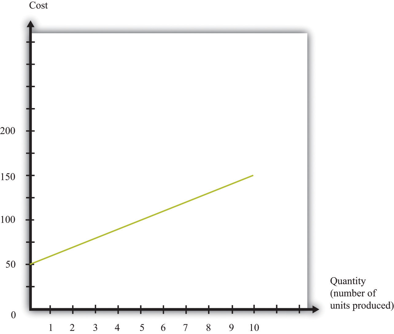
This graph illustrates the cost function for a firm. In this case, the cost function has the equation cost = 50 + 10 × quantity. The cost of producing each additional unit (the marginal cost) is $10.
To emphasize again, only those costs that change matter for a firm’s pricing decision. When a firm considers producing extra output, many of its costs do not change. We can completely ignore these costs when thinking about optimal pricing. This is not to say that other costs don’t matter; quite the contrary. They are critical for a different decision—whether the firm should be in business at all.See Chapter 9 "Growing Jobs". But as long as we are interested in pricing, we can ignore them.
The costs for developing pharmaceutical products are typically quite high. The drug that Ellie was responsible for was first developed in research laboratories, then tested on animals, and then run through a number of clinical studies on human patients. These studies were needed before the Food and Drug Administration in the United States, and equivalent drug safety organizations in other countries, would approve the drug for sale. But these development costs have no effect on marginal cost because they were all incurred before a single pill could be sold.
Surprisingly, this means that even though the drug was very expensive to develop, Ellie’s team—quite correctly—paid no attention to that fact. In determining what price to set, they looked at the price sensitivity of their customers and at marginal cost. They understood that the development costs of the drug were not relevant to the pricing decision. In fact, Ellie’s team had only a very vague idea how much the drug had cost to develop: after all, that development had been carried out by a completely different arm of the company in other parts of the world.
You will often hear the opposite argument. It is common for people to say that pharmaceutical companies charge high prices because it costs so much to develop their drugs. This argument is superficially appealing, but it is completely backward. Pharmaceutical companies don’t charge high prices because they incur large development costs. They are willing to incur large development costs because they can charge high prices.
Estimating Marginal Cost
Estimating marginal cost is generally much easier than estimating demand because the cost side of the business is largely under the control of the firm. The firm’s costs depend on its technology and the decisions made about using that technology. In most medium- or large-sized firms, there is an “operations department” that takes care of the production process. The marketing manager ought to be able to consult with her colleagues in operations and learn about the costs of the firm. Most importantly, even if it is unreasonable to expect an operations manager to know the firm’s entire cost function, the operations manager should have a good idea about marginal cost (that is, should know how much it would cost per unit to scale up operations by a small amount). And that is the information the marketing manager needs for her pricing decisions.
Key Takeaways
- Marginal cost measures the additional costs from producing an extra unit of output.
- It is only the change in costs—marginal cost—that matter for a firm’s pricing decision.
Checking Your Understanding
- If the marginal cost in Table 7.4 "Marginal Cost" were $20, what would be the cost of producing 10 units of the good?
7.4 Markup Pricing: Combining Marginal Revenue and Marginal Cost
Learning Objectives
- What is the optimal price for a firm?
- What is markup?
- What is the relationship between the elasticity of demand and markup?
Let us review the ideas we have developed in this chapter. We know that changes in output lead to changes in both revenues and costs. Changes in revenues and costs lead to changes in profits (see Figure 7.16 "Changes in Revenues and Costs Lead to Changes in Profits"). We have a measure of how much revenues change if output is increased—called marginal revenue, which you can calculate if you know price and the elasticity of demand. We also have a measure of how much costs change if output is increased—this is called marginal cost. Given information on current marginal revenue and marginal cost, a marketing manager can then decide if a firm should change its price. In this section, we derive a rule that tells us how a manager should make this decision.
Figure 7.16 Changes in Revenues and Costs Lead to Changes in Profits
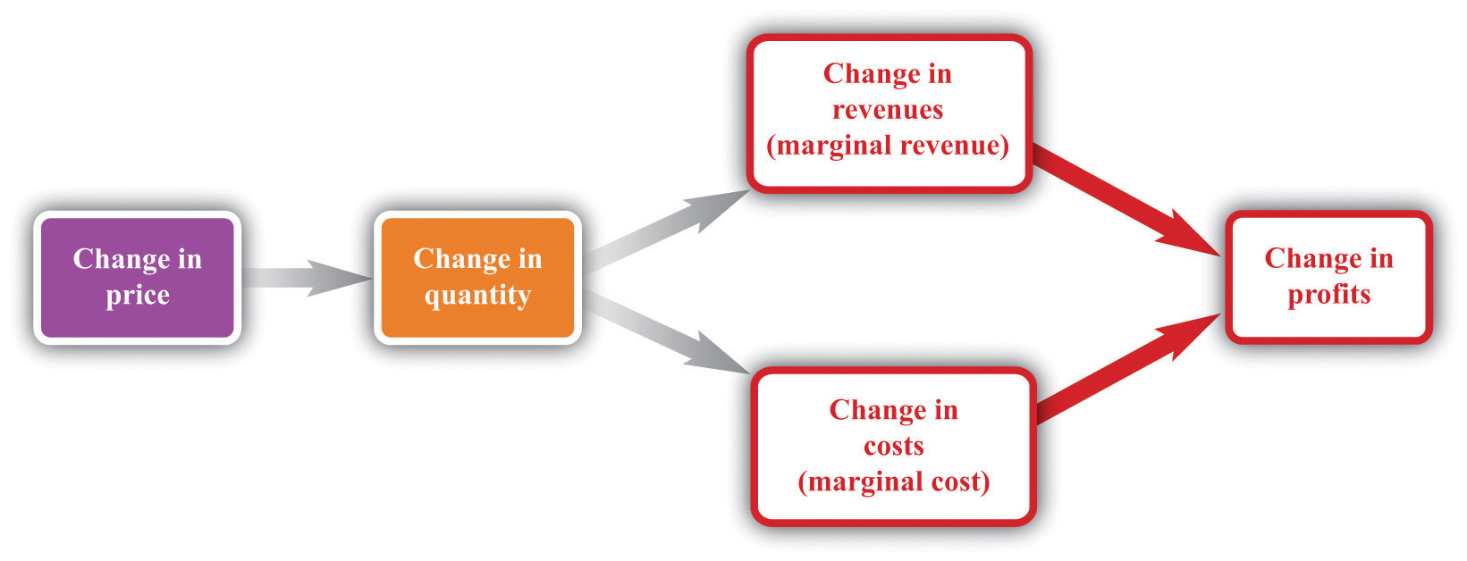
When a firm changes its price, this leads to changes in revenues and costs. The change in a firm’s profit is equal to the change in revenue minus the change in cost—that is, the change in profit is marginal revenue minus marginal cost. When marginal revenue equals marginal cost, the change in profit is zero, so a firm is at the top of the profit hill.
In the real world of business, firms almost always choose the price they set rather than the quantity they produce. Yet the pricing decision is easier to analyze if we think about it the other way round: a firm choosing what quantity to produce and then accepting the price implied by the demand curve. This is just a matter of convenience: a firm chooses a point on the demand curve, and it doesn’t matter if we think about it choosing the price and accepting the implied quantity or choosing the quantity and accepting the implied price (Figure 7.17 "Setting the Price or Setting the Quantity").
Figure 7.17 Setting the Price or Setting the Quantity
It doesn’t matter if we think about choosing the price and accepting the implied quantity or choosing the quantity and accepting the implied price
Suppose that a marketing manager has estimated the elasticity of demand, looked at the current price, and used the marginal revenue formula to discover that the marginal revenue is $5. This means that if the firm increases output by one unit, its revenues will increase by $5. The marketing manager has also spoken to her counterpart in operations, who has told her that the marginal cost is $3. This means it would cost an additional $3 to produce one more unit. From these two pieces of information, the marketing manager knows that an increase in output would be a good idea. An increase in output leads to a bigger increase in revenues than in costs. As a result, it leads to an increase in profits: specifically, profits will increase by $2. This tells the marketing manager that it is a good idea to increase output. From the law of demand, she should think about decreasing the price.
Figure 7.18 Optimal Pricing
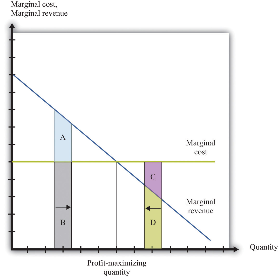
To the left of the point marked “profit-maximizing quantity,” marginal revenue exceeds marginal cost so increasing output is a good idea. The opposite is true to the right of that point.
Figure 7.18 "Optimal Pricing" shows this idea graphically. To the left of the point marked “profit-maximizing quantity,” marginal revenue exceeds marginal cost. Suppose a firm is producing below this level. If it increases its output, the extra revenue it obtains will exceed the extra cost. We see that an increase in output yields extra revenue equal to the areas A + B and extra costs equal to B. The increase in output yields extra profit, which is equal to A. Increasing its output is thus a good idea. Conversely, to the right of the profit-maximizing point, marginal revenue is less than marginal cost. If a firm reduces its output, the decrease in costs (C + D) exceeds the decrease in revenue (D). Decreases in output lead to increases in profit.
Profits are greatest when
marginal revenue = marginal cost.This is the point where a change in price leads to no change in profits, so we are at the very top of the profit hill that we drew in Figure 7.3 "The Profits of a Firm". See also Figure 7.17 "Setting the Price or Setting the Quantity".
The Markup Pricing Formula
Think about Ellie’s company. If it became more expensive for the company to produce each pill, it seems likely they would respond by raising their costs. Also, we said earlier that their customers are not very sensitive to changes in the price, which should allow them to set a relatively high price. In other words, the profit-maximizing price is related to the elasticity of demand and to marginal cost. These are the two critical ingredients of the pricing decision.
Toolkit: Section 31.15 "Pricing with Market Power"
Firms should set the price as a markup over marginal cost:This expression comes from combining the formula for marginal revenue and the condition that marginal revenue equals marginal cost. See the toolkit for more details.
and
There are three facts about markupThe percentage amount by which price exceeds marginal cost.:
- Markup is greater than or equal to zero—that is, the firm never sets a price below marginal cost.
- Markup is smaller when demand is more elastic.
- Markup is zero when the demand curve is perfectly elastic: −(elasticity of demand) = •.
Ellie’s team looked at their numbers. At the current price, −(elasticity of demand) = 1.47. They learned that the marginal cost was $0.28 per pill, and they were charging $0.50 per pill. Their current markup, in other words, was about 79 percent: 0.5 = (1+ 0.79) × 0.28. But if they applied the markup pricing formula based on the current elasticity of demand, they could charge a markup of 1/0.47 = 2.12—that is, more than a 200 percent markup, leading to a price of $0.87. It was clear that they could do better by increasing their price
A Pricing Algorithm
To summarize, a manager needs two key pieces of information when determining price:
- Marginal cost. We have shown that the profit-maximizing price is a markup over the marginal cost of production. If a manager does not know the magnitude of marginal cost, she is missing a critical piece of information for the pricing decision.
- Elasticity of demand. Once a manager knows marginal cost, she should then set the price as a markup over marginal cost. But this should not be done in an ad hoc manner; the markup must be based on information about the elasticity of demand.
Given these two pieces of information, a manager can then use the markup formula to determine the optimal price. Be careful, though. The markup formula looks deceptively simple, as if it can be used in a “plug-and-play” manner—given marginal cost and the elasticity of demand, plug them into the formula and calculate the optimum price. But if you change the price, both marginal cost and the elasticity of demand are also likely to change. A more reliable way of using this formula is in the algorithm shown in Figure 7.19 "A Pricing Algorithm", which is based on our earlier idea that you should find your way to the top of the profit hill. The five steps are as follows:
- At your current price, estimate marginal cost and the elasticity of demand.
- Calculate the optimal price based on those values.
- If the optimal price is greater than your actual price, increase your price. Then estimate marginal cost and the elasticity again and repeat the process.
- If the optimal price is less than your actual price, decrease your price. Then estimate marginal cost and the elasticity again and repeat the process.
- If the current price is equal to this optimal price, leave your price unchanged.
Figure 7.19 A Pricing Algorithm
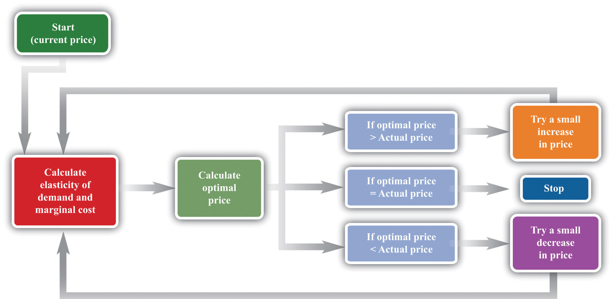
This pricing algorithm shows how to get the best price for a product.
Ellie’s team members were aware that, even though demand for the drug was apparently not very sensitive to price, they should not immediately jump to a much higher markup. They had found that based on current marginal cost and elasticity, the price could be raised. But as they raised the price, they knew that the elasticity of demand would probably also change. Looking more closely at their market research data, they found that at a price of $0.56 (a 100 percent markup), the elasticity of demand would increase to about 2. An elasticity of 2 means that the markup should be 100 percent to maximize profits. Thus—at least if their market research data were reliable—they knew that a price of $0.56 would maximize profits. Ellie recommended to senior management that the price of the drug be raised by slightly over 10 percent, from $0.50 per pill to $0.56 per pill.
Shifts in the Demand Curve Facing a Firm
So far we have looked only at movements along the demand curve—that is, we have looked at how changes in price lead to changes in the quantity that customers will buy. Firms also need to understand what factors might cause their demand curve to shift. Among the most important are the following:
- Changes in household tastes. Starting around 2004 or so, low-carbohydrate diets started to become very popular in the United States and elsewhere. For some companies, this was a boon; for others it was a problem. For example, companies like Einstein Bros. Bagels or Dunkin’ Donuts sell products that are relatively high in carbohydrates. As more and more customers started looking for low-carb alternatives, these firms saw their demand curve shift inward.
- Business cycle. Consider Lexus, a manufacturer of high-end automobiles. When the economy is booming, sales are likely to be very good. In boom times, people feel richer and more secure and are more likely to purchase a luxury car. But if the economy goes into recession, potential car buyers will start looking at cheaper cars or may decide to defer their purchase altogether. Many companies sell products that are sensitive to the state of the business cycle. Their demand curves shift as the economy moves from boom to recession.
- Changes in competitors’ prices. In a business setting, this is a critical concern. If a competitor decreases its price, this means that the demand curve you face will shift inward. For example, suppose that British Airways decides to decrease its price for flights from New York to London. American Airlines will find that its demand curve for that route has shifted inward. Ellie certainly has to worry about this because her company’s product has only a small number of competitors. A change in price of a competing blood pressure drug might make a big difference in the sales and profits of Ellie’s product.
If the demand curve shifts, should a firm change its price? The answer is yes if the shift in the demand curve also leads to a change in the elasticity of demand. In practice, this is likely to be the case, although it is certainly possible for a demand curve to shift without a change in the elasticity of demand. The correct response to a shift in the demand curve is to reestimate the elasticity of demand and then decide if a change in price is appropriate.
Complications
Pricing is a difficult and delicate job, and there are many factors that we have not yet considered:We address some of them in other chapters of the book; others are topics for more advanced classes in economics and business strategy.
- By far the most important problem that we have neglected is as follows: When making pricing decisions, firms may need to take into account how other firms will respond to their decisions. For example, a manager might estimate her firm’s elasticity of demand and marginal cost and determine that she could make more money by decreasing price. That calculation presumes that competing firms keep their prices unchanged. In markets with a small number of competitors, it is instead quite likely that other firms would respond by decreasing their prices. This would cause a firm’s demand curve to shift inward and probably leave it worse off than before.
- We have assumed throughout that a firm has to charge the same price for every unit that it sells. In many cases, this is an accurate description of pricing behavior. When a grocery store posts a price, that price holds for every unit on the shelf. But sometimes firms charge different prices for different units—by either charging different prices to different customers or offering individual units at different prices to the same customer. You have undoubtedly encountered examples. Firms sometimes offer quantity discounts, so the price is lower if you buy more units. Sometimes they offer discounts to certain groups of customers, such as cheap movie tickets for students. We could easily fill an entire chapter with other examples—some of which are remarkably sophisticated.
- Firms can have pricing strategies that call for the price to change over time. For example, firms sometimes engage in a strategy known as penetration pricing, whereby they start off by charging a low price in an attempt to develop or expand the market. Imagine that Kellogg’s develops a new breakfast cereal. It might decide to offer the cereal at a low price to induce people to try the product. Only after it has developed a group of loyal customers would it start setting their prices according to the markup principle.
- Pricing plays a role in the overall marketing and branding strategy of a firm. Some firms position themselves in the marketplace as suppliers of high-end offerings. They may choose to set high prices for their products to ensure that customers perceive them appropriately. Consider a luxury hotel that is contemplating setting a very low price in the off-season. Even though such a strategy might make sense in terms of its profits at that time, it might do long-term damage to the hotel’s reputation. For various reasons, customers often use the price of a product as an indicator of that product’s quality, so a low price can adversely affect a firm’s image.
- Psychologists who study marketing have found that demand is sensitive at certain price points. For example, if a firm increases the price of a product from $99.98 to $99.99, there might be very little effect on demand. But if the price increases from $99.99 to $100.00, there might be a much bigger effect because $100.00 is a psychological barrier. Such consumer behavior does not seem completely rational, but there is little doubt that it is a real phenomenon.
- Throughout this chapter, we have said that there is no difference between a firm choosing its price and taking as given the implied quantity or choosing its quantity and taking as given the implied price. Either way, the firm is picking a point on the demand curve. This is true, but there is a footnote that we should add. A firm’s demand curve depends on what its competitors are doing and, oddly enough, it does make a difference if those competitors are choosing quantities or prices.See Chapter 15 "Busting Up Monopolies" for discussion of this. We should also note that firms often do not know their demand curves with complete certainty. Suppose, for example, that the true demand curve for a firm’s product is actually further outward than a firm expects. If the firm sets the price, it will end up with an unexpectedly large quantity being demanded. If the firm sets the quantity, it will end up with an unexpectedly high price.
- We have focused our attention on the market power of firms as sellers, as reflected in the downward-sloping demand curves they face. Firms can also have market power as buyers. Walmart is such an important customer for many of its suppliers that it can use its position to negotiate lower prices for the goods it buys. Governments are also often powerful buyers and may be able to influence the prices they pay for goods and services. For example, government-run health-care systems may be able to negotiate favorable prices with pharmaceutical companies.
Key Takeaways
- At the profit-maximizing price, marginal revenue equals marginal cost.
- Markup is the difference between price and marginal cost, as a percentage of marginal cost.
- The more elastic the demand curve faced by a firm, the smaller the markup.
Checking Your Understanding
- We said that markup is always greater than zero. Look at the formula for markup. If markup is greater than zero, what must be true about −(elasticity of demand)? Can you see why this must be true? Look back at Figure 7.13 "Marginal Revenue and the Elasticity of Demand" for a hint.
- If price is a markup over marginal cost, then how does marginal revenue influence the pricing decision of a firm?
- Starting at the profit-maximizing price, if a firm increases its price, could revenue increase?
7.5 The Supply Curve of a Competitive Firm
Learning Objectives
- What is a perfectly competitive market?
- In a perfectly competitive market, what does the demand curve faced by a firm look like?
- What happens to the pricing decision of a firm in a perfectly competitive market?
In this chapter, we have paid a great deal of attention to demand, but we have not spoken of supply. There is a good reason for this: a firm with market power does not have a supply curve. A supply curve for a firm tells us how much output the firm is willing to bring to market at different prices. But a firm with market power looks at the demand curve that it faces and then chooses a point on that curve (a price and a quantity). Price, in this chapter, is something that a firm chooses, not something that it takes as given. What is the connection between our analysis in this chapter and a market supply curve?
Perfectly Competitive Markets
If you produce a good for which there are few close substitutes, you have a great deal of market power. Your demand curve is not very elastic: even if you charge a high price, people will be willing to buy the good. On the other hand, if you are the producer of a good that is very similar to other products on the market, then your demand curve will be very elastic. If you increase your price even a little, the demand for your product will decrease a lot.
The extreme case is called a perfectly competitive market. In a perfectly competitive market, there are numerous buyers and sellers of exactly the same good. The standard examples of perfectly competitive markets are those for commodities, such as copper, sugar, wheat, or coffee. One bushel of wheat is the same as another, there are many producers of wheat in the world, and there are many buyers. Markets for financial assets may also be competitive. One euro is a perfect substitute for another, one three-month US treasury bill is a perfect substitute for another, and there are many institutions willing to buy and sell such assets.
Toolkit: Section 31.9 "Supply and Demand"
You can review the market supply curve and the definition of a perfectly competitive market in the toolkit.
An individual seller in a competitive market has no control over price. If the seller tries to set a price above the going market price, the quantity demanded falls to zero. However, the seller can sell as much as desired at the market price. When there are many sellers producing the same good, the output of a single seller is tiny relative to the whole market, and so the seller’s supply choices have no effect on the market price. This is what we mean by saying that the seller is “small.” It follows that a seller in a perfectly competitive market faces a demand curve that is a horizontal line at the market price, as shown in Figure 7.20 "The Demand Curve Facing a Firm in a Perfectly Competitive Market". This demand curve is infinitely elastic: −(elasticity of demand) = ∞. Be sure you understand this demand curve. As elsewhere in the chapter, it is the demand faced by an individual firm. In the background, there is a market demand curve that is downward sloping in the usual way; the market demand and market supply curves together determine the market price. But an individual producer does not experience the market demand curve. The producer confronts an infinitely elastic demand for its product.
Figure 7.20 The Demand Curve Facing a Firm in a Perfectly Competitive Market
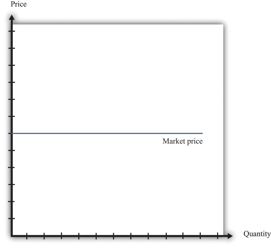
The demand curve faced by a firm in a perfectly competitive market is infinitely elastic. Graphically, this means that it is a horizontal line at the market price.
Everything we have shown in this chapter applies to a firm facing such a demand curve. The seller still picks the best point on the demand curve. But because the price is the same everywhere on the demand curve, picking the best point means picking the best quantity. To see this, go back to the markup formula. When demand is infinitely elastic, the markup is zero:
so price equals marginal cost:
price = (1 + markup) × marginal cost = marginal cost.This makes sense. The ability to set a price above marginal cost comes from market power. If you have no market power, you cannot set a price in excess of marginal cost. A perfectly competitive firm chooses its level of output so that its marginal cost of production equals the market price.
We could equally get this conclusion by remembering that
marginal revenue = marginal costand that when −(elasticity of demand) is infinite, marginal revenue equals price. If a competitive firm wants to sell one more unit, it does not have to decrease its price to do so. The amount it gets for selling one more unit is therefore the market price of the product, and the condition that marginal revenue equals marginal cost becomes
price = marginal cost.For the goods and services that we purchase regularly, there are few markets that are truly perfectly competitive. Often there are many sellers of goods that may be very close substitutes but not absolutely identical. Still, many markets are close to being perfectly competitive, in which case markup is very small and perfect competition is a good approximation.
The Supply Curve of a Firm
Table 7.5 "Costs of Production: Increasing Marginal Cost" shows the costs of producing for a firm. In contrast to Table 7.4 "Marginal Cost", where we supposed marginal cost was constant, this example has higher marginal costs of production when the level of output is greater.Total cost in Table 7.5 "Costs of Production: Increasing Marginal Cost" is 50 + 10 × quantity + 2 × quantity2.
Table 7.5 Costs of Production: Increasing Marginal Cost
| Output | Total Costs ($) | Marginal Cost ($) |
|---|---|---|
| 1 | 22 | 12 |
| 2 | 38 | 16 |
| 3 | 58 | 20 |
| 4 | 82 | 24 |
| 5 | 110 | 28 |
| … |
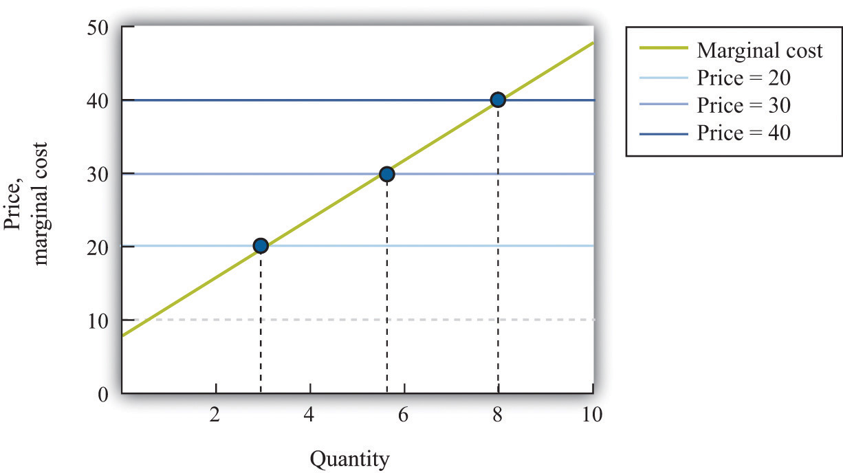
Figure 7.21 "The Supply Curve of an Individual Firm" shows how we derive the supply curve of an individual firm given such data on costs. The supply curve tells us how much the firm will produce at different prices. Suppose, for example, that the price is $20. At this price, we draw a horizontal line until we reach the marginal cost curve. At that point, we draw a vertical line to the quantity axis. In this way, you can find the level of output such that marginal cost equals price. Looking at the figure, we see that the firm should produce 3 units because the marginal cost of producing the third unit is $20. When the price is $30, setting marginal cost equal to price requires the firm to produce 5.5 units. When the price is $40, setting marginal cost equal to price requires the firm to produce 8 units.
The supply curve shows us the quantity that a firm will produce at different prices. Figure 7.21 "The Supply Curve of an Individual Firm" reveals something remarkable: the individual supply curveHow much output a firm in a perfectly competitive market will supply at any given price. It is the same as a firm’s marginal cost curve. of the firm is the marginal cost curve. They are the same thing. As the price a firm faces increases, it will produce more. Note carefully how this is worded. We are not saying that if a firm produces more, it will charge a higher price. Firms in a competitive market must take the price as given. Instead, we think about the response of a firm to a change in the price.The individual firm’s supply curve is an exact counterpart to something we show in Chapter 4 "Everyday Decisions", where we derive the demand curve for an individual. We show that an individual buys a good up to the point where marginal valuation equals price. From this we can conclude that the demand curve for an individual is the same as the individual’s marginal valuation curve. In Chapter 8 "Why Do Prices Change?", we use an individual firm’s supply curve as the basis for the market supply curve. Likewise, we use the individual demand curve as the basis for the market demand curve. By combining these curves, we obtain the supply-and-demand framework, which we can use to understand changing prices in an economy.
Toolkit: Section 31.9 "Supply and Demand"
The individual supply curve shows how much output a firm in a perfectly competitive market will supply at any given price. Provided that a firm is producing output, the supply curve is the same as marginal cost curve.
Figure 7.21 The Supply Curve of an Individual Firm
The firm chooses its quantity such that price equals marginal cost, which implies that the marginal cost curve of the firm is the supply curve of the firm.
Key Takeaways
- A perfectly competitive market has a large number of buyers and sellers of exactly the same good.
- In a perfectly competitive market, an individual firm faces a demand curve with infinite elasticity.
- In a perfectly competitive market, the firm does not set a price but chooses a level of output such that marginal cost equals the market price.
Checking Your Understanding
- Explain why the demand curve a firm faces in a perfectly competitive market is horizontal even though the market demand curve is not horizontal.
- Why is the cost of one unit $60 in Table 7.4 "Marginal Cost" but only $22 in Table 7.5 "Costs of Production: Increasing Marginal Cost"?
7.6 End-of-Chapter Material
In Conclusion
Choosing the right price is one of the hardest problems that a manager faces. It is also one of the most consequential: few other decisions have such immediate impact on the health and success of a firm. It is hardly surprising that firms devote considerable resources to deciding on the price to set. Even though firms operate in many different market settings, our analysis of markup pricing is very general: it applies to firms in all sorts of different circumstances. It is thus a powerful tool for understanding the behavior of firms in an economy.
One goal of this textbook is to help you make good decisions, both in your everyday life and in your future careers. In this chapter, we have set out the principles of how prices should be set, assuming that the goal of a manager is to make as much profit for a firm as possible. It does not necessarily follow, however, that this is how managers actually behave in real life. Does this chapter just describe a make-believe world of economists or does it also describe how prices are set in the real business world?
The answer is a bit of both. Managers must think carefully about costs and demand when setting prices. Market research firms routinely investigate consumers’ price sensitivities and estimate elasticities. At the same time, pricing decisions are sometimes more haphazard than this chapter might suggest. In practice, managers often use rules of thumb or standard markups that are not necessarily solidly based on the elasticity of demand.
There is one reason to think that managers do not stray too far from the prices that maximize their firms’ profits, however. Business is a competitive affair, and firms that make poor decisions will often not survive in the marketplace. If a firm consistently sets the wrong price, it will make less money than its competitors and will probably be forced out of business or taken over by another firm that can do a better job of management. The marketplace imposes a harsh discipline on badly managed firms, but the end result is—usually at least—a more efficient and better-functioning economy.
Key Link
- College pricing: http://www.collegeboard.com/student/pay/add-it-up/4494.html
Exercises
-
We suggested that a grocery store could conduct an experiment to find a demand curve by charging a different price each week for some product.
- Do you think that technique would be more accurate for a perishable good, such as milk, or for a nonperishable good, such as canned tuna? Why?
- Do you think the technique would be more accurate if the firm announced the price each week in advance or if it just let customers discover the different prices when they came to the store? Why?
- Extend Table 7.5 "Costs of Production: Increasing Marginal Cost" for output levels 6–10. What does Table 7.5 "Costs of Production: Increasing Marginal Cost" look like if the fixed cost is $100?
- Suppose your company is selling a product that is an inferior good. What do you think will happen to the demand curve facing your firm when the economy goes into recession?
- Suppose you are a producer of DVDs and imagine that producers of DVD players decrease their prices. What do you think will happen to the demand curve you face?
- If you were running a fast-food restaurant, what factors would you take into account in setting a price for burgers?
- Suppose a monopolist could produce an extra unit at zero marginal cost and, at the current price, faces a demand curve with an −(elasticity of demand) of 2. Should the monopolist raise or lower its price to make more profit?
- Suppose that instead of maximizing profit, the monopolist in Question 6 wants to maximize revenues. Would it behave any differently? What if the marginal cost was positive?
- If the price of steak is $25.00 a pound and the −(elasticity of demand) is 2, what decrease in price would lead the quantity sold to increase by 4 percent?
- Explain why marginal revenue must be less than the price when a firm faces a downward-sloping demand curve.
- A monopolist is maximizing profit. Perhaps due to an innovation in some other product line, he finds that the elasticity of demand for his product is lower. What will this change in the elasticity of demand due to the profit of the monopolist? How will the monopolist respond to this change?
-
The following is an excerpt from an article in the Singaporean newspaper, the Straits Times:
Singaporeans with a sweet tooth could soon find themselves paying more for their favourite treats, as bakers and confectioners buckle under soaring sugar prices.
Since March last year, the price of white sugar has shot up by 70 per cent, according to the New York Board of Trade. As if that didn’t make life difficult enough for bakers, butter and cheese prices have also risen, by 31 per cent and 17 per cent respectively.
The increases have been caused by various factors: a steep drop in Thailand’s sugarcane production due to drought, higher sea freight charges, increasing demand from China’s consumers for dairy products and the strong Australian and New Zealand dollar.
For the consumer in Singapore, what this may eventually boil down to is a more expensive bag of cookies, with prices at some bakeries expected to rise between 10 and 20 per cent.
[The owner of a Singapore bakery, Mr. Leong Meng Pock], said that he intends to raise prices possibly as early as next month. A sugared doughnut at his shop sells for 50 cents [about US$0.30] and a slice of Black Forest cake for $1.80 [about US$1.13], prices that have remained unchanged since 1990. Next month, the doughnuts may go up to 60 cents and the Black Forest cake to $2.
Said Mr Leong: “In Singapore, you have bread and cake prices that are at least 10 years old. This is especially true for the HDB [government-subsidized housing] neighborhoods, where customers are very price-sensitive.”See http://straitstimes.asia1.com.sg.
- Do you think bakers face a demand curve that is relatively elastic or relatively inelastic? Why?
- What has happened to their marginal cost?
- Explain the difference between a shift in the demand curve and movement along a demand curve.
- If you observe the price of a product, then you can infer the marginal cost of the product if and only if the market is competitive. Explain.
Spreadsheet Exercise
- Suppose that the cost function for a product is given by total costs = 100 + 2,000 × quantity. Create a spreadsheet to calculate the costs for different levels of output and use it to produce a graph like Figure 7.16 "Changes in Revenues and Costs Lead to Changes in Profits".
Economics Detective
- What prices are your local gas stations currently charging for gas? Do the stations generally have the same price for gas? If not, what would explain the differences in prices they set? Do the stations charge the same price all the time or does the price change? When the price changes, what might be the reason for that change?
- Think about the college you are attending. What determines the profit of the college—what are its revenues and what are its costs? What is tuition at your college? Would you advocate an increase or a decrease in tuition rates to increase revenue at your college? What factors determine the elasticity of demand faced by your college?