This is “The Ricardian Model Production Possibility Frontier”, section 2.4 from the book Policy and Theory of International Trade (v. 1.0). For details on it (including licensing), click here.
For more information on the source of this book, or why it is available for free, please see the project's home page. You can browse or download additional books there. To download a .zip file containing this book to use offline, simply click here.
2.4 The Ricardian Model Production Possibility Frontier
Learning Objective
- Learn how the plot of the labor constraint yields the production possibility frontier.
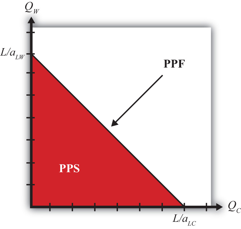
Using the two production functions and the labor constraint, we can describe the production possibility frontier (PPF)The set of all output combinations that could be produced in a country when all the labor inputs are fully employed. In the Ricardian model, the PPF is linear.. First, note that the production functions can be rewritten as LC = aLC QC and LW = aLW QW. Plugging these values for LC and LW into the labor constraint yields the equation for the PPF:
aLC QC + aLW QW = L.This equation has three exogenous variables (aLC, aLW, and L) that we assume have known values and two endogenous variables (QC and QW) whose values must be solved for. The PPF equation is a linear equation—that is, it describes a line. With some algebraic manipulation, we can rewrite the PPF equation into the standard form for an equation of a line, generally written as y = mx + b, where y is the variable on the vertical axis, x is the variable on the horizontal axis, m is the slope of the line, and b is the y-intercept. The PPF equation can be rewritten as
We plot the PPF on the diagram in Figure 2.1 "Production Possibilities" with QC on the horizontal axis and QW on the vertical axis. The equation is easily plotted by following three steps.
Figure 2.1 Production Possibilities

- Set QC = 0 and solve for QW. In this case, the solution is . This corresponds to the QW-intercept. It tells us the quantity of wine that the United States could produce if it devoted all of its labor force (L) to the production of wine.
- Set QW = 0 and solve for QC. In this case, the solution is . This corresponds to the QC-intercept. It tells us the quantity of cheese that the United States could produce if it devoted all of its labor force (L) to the production of cheese.
- Connect the two points with a straight line.
The straight downward-sloping line is the production possibility frontier. It describes all possible quantity combinations of wine and cheese that can be achieved by the U.S. economy. A movement along the curve represents a transfer of labor resources out of one industry and into another such that all labor remains employed.
Points inside the PPF are production possibilities but correspond to underemployment of labor resources. In fact, all production possibilities regardless of whether full employment is fulfilled are referred to as the production possibility set (PPS). The PPS is represented by all the points within and on the border of the red triangle in Figure 2.1 "Production Possibilities".
Key Takeaways
- The equation aLC QC + aLW QW = L is an equation of a line whose plot represents the country’s production possibility frontier (PPF).
- A PPF is the combination of outputs of cheese and wine that the country can produce given a production technology (i.e., given that unit labor requirements are exogenous) and assuming all of its labor hours are employed.
- A production possibility set (PPS) is the combination of outputs that a country can produce even if some of the labor is unemployed.
Exercises
-
Jeopardy Questions. As in the popular television game show, you are given an answer to a question and you must respond with the question. For example, if the answer is “a tax on imports,” then the correct question is “What is a tariff?”
- The term describing the set of all output combinations that can be produced within an economy.
- The term describing the set of all output combinations that can be produced within an economy with full employment of all available resources.
- Suppose that the unit labor requirements for wine and cheese are aLC = 6 hrs./lb., aLW = 4 hrs./gal., respectively, and that total labor hours available for production are 60. What is the maximum output of cheese? What is the maximum output of wine?
- Suppose that the unit labor requirements for wine and cheese are aLC = 6 hrs./lb. and aLW = 4 hrs./gal., respectively, and that total labor hours available for production are 60. Plot the production possibility frontier.


