This is “Surface Analysis: Spatial Interpolation”, section 8.3 from the book Geographic Information System Basics (v. 1.0). For details on it (including licensing), click here.
For more information on the source of this book, or why it is available for free, please see the project's home page. You can browse or download additional books there. To download a .zip file containing this book to use offline, simply click here.


8.3 Surface Analysis: Spatial Interpolation
Learning Objective
- The objective of this section is to become familiar with concepts and terms related to GIS surfaces, how to create them, and how they are used to answer specific spatial questions.
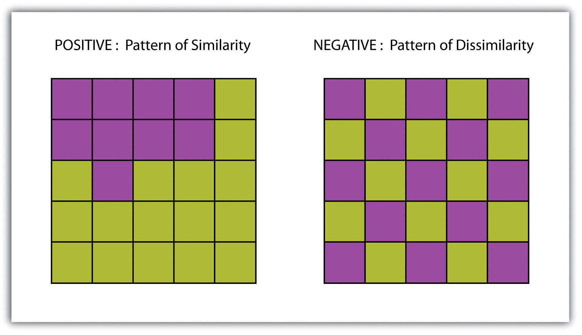
A surfaceA vector or raster dataset that contains an attribute value for every locale throughout its extent. is a vector or raster dataset that contains an attribute value for every locale throughout its extent. In a sense, all raster datasets are surfaces, but not all vector datasets are surfaces. Surfaces are commonly used in a geographic information system (GIS) to visualize phenomena such as elevation, temperature, slope, aspect, rainfall, and more. In a GIS, surface analyses are usually carried out on either raster datasets or TINs (Triangular Irregular Network; Chapter 5 "Geospatial Data Management", Section 5.3.1 "Vector File Formats"), but isolines or point arrays can also be used. Interpolation is used to estimate the value of a variable at an unsampled location from measurements made at nearby or neighboring locales. Spatial interpolation methods draw on the theoretical creed of Tobler’s first law of geography, which states that “everything is related to everything else, but near things are more related than distant things.” Indeed, this basic tenet of positive spatial autocorrelationThe result of similar values occurring near by each other. forms the backbone of many spatial analyses (Figure 8.9 "Positive and Negative Spatial Autocorrelation").
Figure 8.9 Positive and Negative Spatial Autocorrelation
Creating Surfaces
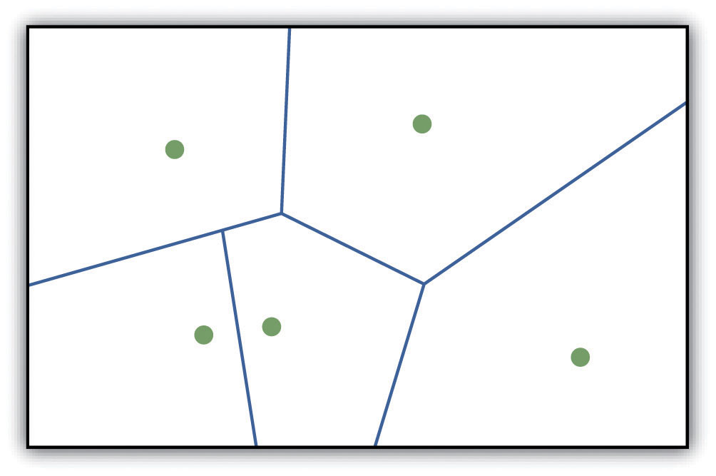
The ability to create a surface is a valuable tool in a GIS. The creation of raster surfaces, however, often starts with the creation of a vector surface. One common method to create such a vector surface from point data is via the generation of Thiessen (or Voronoi) polygons. Thiessen polygons are mathematically generated areas that define the sphere of influence around each point in the dataset relative to all other points (Figure 8.10 "A Vector Surface Created Using Thiessen Polygons"). Specifically, polygon boundaries are calculated as the perpendicular bisectors of the lines between each pair of neighboring points. The derived Thiessen polygons can then be used as crude vector surfaces that provide attribute information across the entire area of interest. A common example of Thiessen polygons is the creation of a rainfall surface from an array of rain gauge point locations. Employing some basic reclassification techniques, these Thiessen polygons can be easily converted to equivalent raster representations.
Figure 8.10 A Vector Surface Created Using Thiessen Polygons
While the creation of Thiessen polygons results in a polygon layer whereby each polygon, or raster zone, maintains a single value, interpolationA potentially complex statistical technique that estimates the value of all unknown points between the known points. is a potentially complex statistical technique that estimates the value of all unknown points between the known points. The three basic methods used to create interpolated surfaces are spline, inverse distance weighting (IDW), and trend surface. The spline interpolation method forces a smoothed curve through the set of known input points to estimate the unknown, intervening values. IDW interpolation estimates the values of unknown locations using the distance to proximal, known values. The weight placed on the value of each proximal value is in inverse proportion to its spatial distance from the target locale. Therefore, the farther the proximal point, the less weight it carries in defining the target point’s value. Finally, trend surface interpolation is the most complex method as it fits a multivariate statistical regression model to the known points, assigning a value to each unknown location based on that model.
Other highly complex interpolation methods exist such as kriging. KrigingA complex geostatistical technique that employs semivariograms to interpolate the values of an input point layer and is more akin to a regression analysis. is a complex geostatistical technique, similar to IDW, that employs semivariograms to interpolate the values of an input point layer and is more akin to a regression analysis (Krige 1951).Krige, D. 1951. A Statistical Approach to Some Mine Valuations and Allied Problems at the Witwatersrand. Master’s thesis. University of Witwatersrand. The specifics of the kriging methodology will not be covered here as this is beyond the scope of this text. For more information on kriging, consult review texts such as Stein (1999).Stein, M. 1999. Statistical Interpolation of Spatial Data: Some Theories for Kriging. New York: Springer.
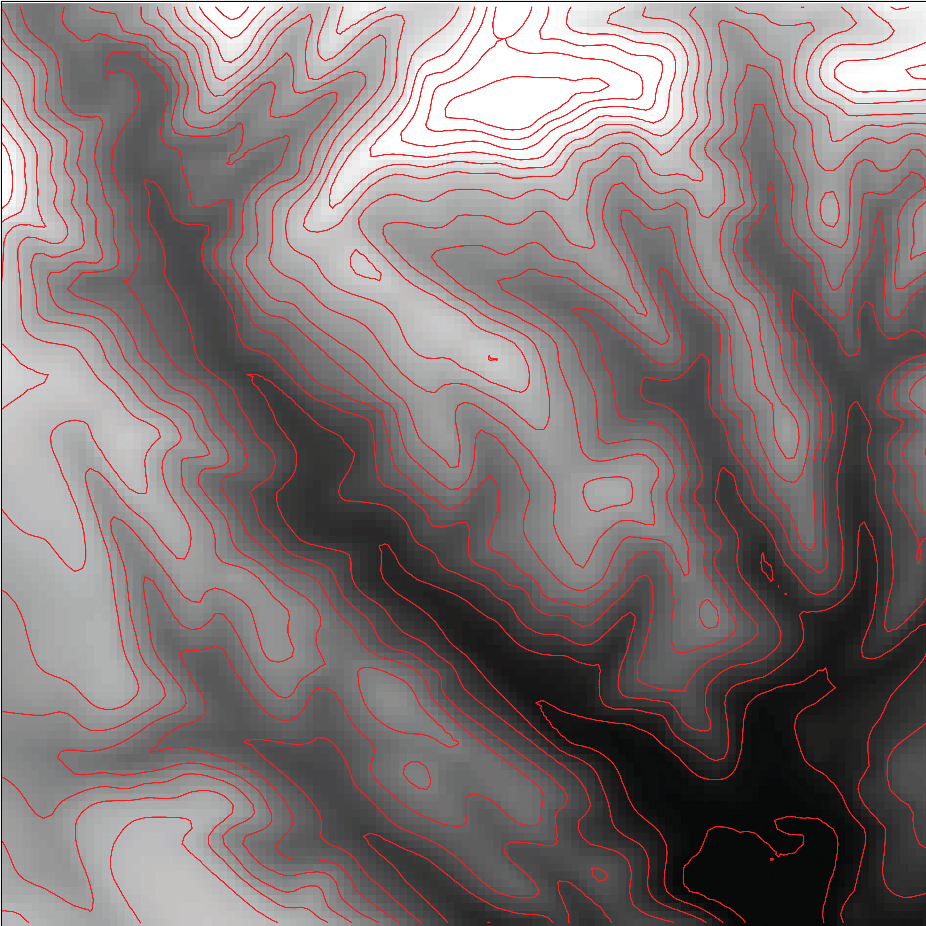
Inversely, raster data can also be used to create vector surfaces. For instance, isoline maps are made up of continuous, nonoverlapping lines that connect points of equal value. Isolines have specific monikers depending on the type of information they model (e.g., elevation = contour lines, temperature = isotherms, barometric pressure = isobars, wind speed = isotachs) Figure 8.11 "Contour Lines Derived from a DEM" shows an isoline elevation map. As the elevation values of this digital elevation model (DEM) range from 450 to 950 feet, the contour lines are placed at 500, 600, 700, 800, and 900 feet elevations throughout the extent of the image. In this example, the contour interval, defined as the vertical distance between each contour line, is 100 feet. The contour interval is determined by the user during the creating of the surface.
Figure 8.11 Contour Lines Derived from a DEM
Key Takeaways
- Spatial interpolation is used to estimate those unknown values found between known data points.
- Spatial autocorrelation is positive when mapped features are clustered and is negative when mapped features are uniformly distributed.
- Thiessen polygons are a valuable tool for converting point arrays into polygon surfaces.
Exercises
- Give an example of five phenomena in the real world that exhibit positive spatial autocorrelation.
- Give an example of five phenomena in the real world that exhibit negative spatial autocorrelation.