This is “Aggregate Demand”, section 23.1 from the book Finance, Banking, and Money (v. 1.1). For details on it (including licensing), click here.
For more information on the source of this book, or why it is available for free, please see the project's home page. You can browse or download additional books there. To download a .zip file containing this book to use offline, simply click here.
23.1 Aggregate Demand
Learning Objectives
- What is the AD curve and why does it slope downward?
- What shifts the AD curve and why?
We learned in Chapter 22 "IS-LM in Action" that the IS-LM model isn’t entirely agreeable to policymakers because it examines only the short term, and when pressed into service for the long-term, or changes in the price level, it suggests that policy initiatives are more likely to mess matters up than to improve them. In response, economists developed a new theory, aggregate demand and supply, that relates the price level to the total final goods and services demanded (aggregate demand [AD]) and the total supplied (aggregate supply [AS]). This new framework is attractive for several reasons: (1) it can be used to examine both the short and the long run; (2) it takes a form similar to the microeconomic price theory model of supply and demand, so it is familiar; and (3) it gives policymakers some grounds for implementing activist economic policies. To understand aggregate demand and supply theory, we need to understand how each of the curves is derived.
The aggregate demand curve can be derived three ways, through the IS-LM model as described at the end of Chapter 22 "IS-LM in Action", with help from the quantity theory of money, or directly from its components. Remember that Y = C + I + G + NX. As the price level falls, ceteris paribus, real money balances are higher. That spells a lower interest rate, as we learned in Chapter 5 "The Economics of Interest-Rate Fluctuations". A lower interest rate, in turn, means an increase in I (and hence Y). A lower interest rate also means a lower exchange rate and, as explained in Chapter 18 "Foreign Exchange", more exports and fewer imports. So NX also increases. (C might be positively affected by lower i as well.) As the price level increases, the opposite occurs. So the AD curve slopes downward.
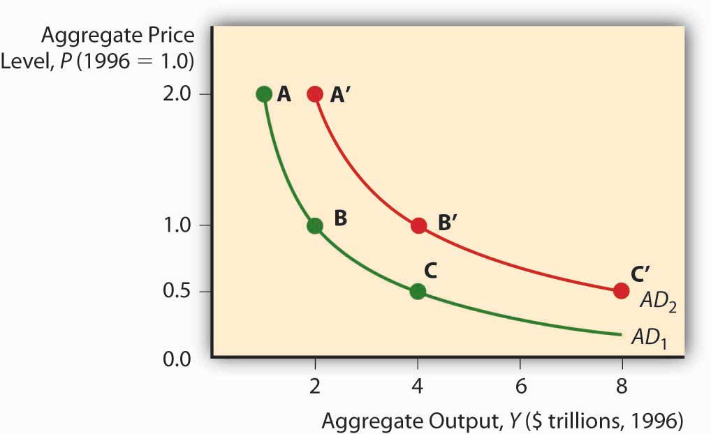
Figure 23.1 Aggregate demand curve

The quantity theory of money also shows that the AD curve should slope downward. Remember that the quantity theory ties money to prices and output via velocity, the average number of times annually a unit of currency is spent on final goods and services, in the so-called equation of exchange:
where
M = money supply
V = velocity of money
P = price level
Y = aggregate output
If M = $100 billion and V = 3, then PY must be $300 billion. If we set P, the price level, equal to 1, Y must equal $300 billion (300/1). If P is 2, then Y is $150 billion (300/2). If it is .5, then Y is $600 billion (300/.5). Plot those points and you get a downward sloping curve, as in Figure 23.1 "Aggregate demand curve". The AD curve shifts right if the MS increases and left if it decreases. Continuing the example above, if we hold P constant at 1.0 but double M to $200 billion, then Y will double to $600 billion (200 × 3). (Recall that the theory suggests that V changes only slowly.) Cut M in half ($50 billion) and Y will fall by half, to $150 billion (50 × 3).
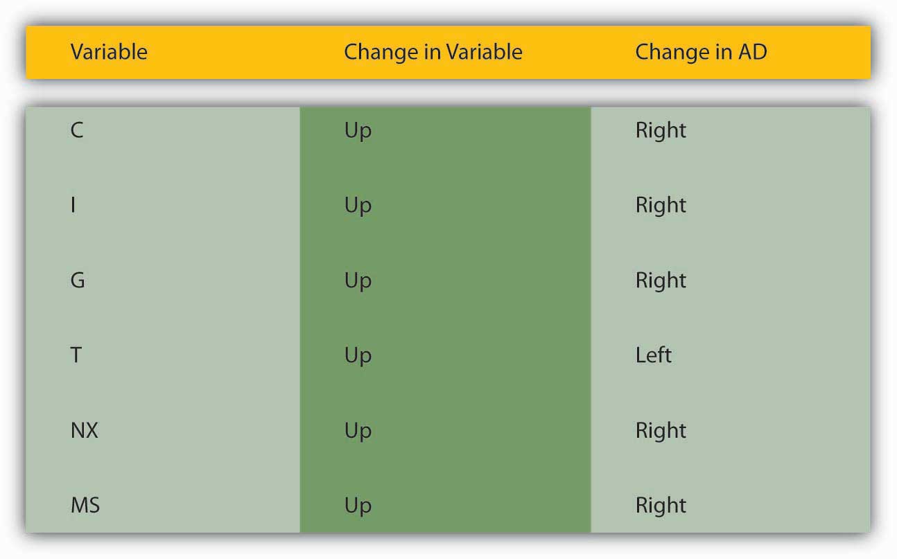
Figure 23.2 Factors that shift the aggregate demand curve

For a summary of the factors that shift the AD curve, review Figure 23.2 "Factors that shift the aggregate demand curve".
Key Takeaways
- The aggregate demand (AD) curve is the total quantity of final goods and services demanded at different price levels.
- It slopes downward because a lower price level, holding MS constant, means higher real money balances.
- Higher real money balances, in turn, mean lower interest rates, which means more investment (I) due to more +NPV projects and more net exports (NX) due to a weaker domestic currency (exports increase and imports decrease).
- The AD curve is positively related to changes in MS, C, I, G, and NX, and is negatively related to T.
- Those variables shift AD for the same reasons they shift Yad and the IS curve, as discussed in Chapter 21 "IS-LM" and Chapter 22 "IS-LM in Action", because all of them except taxes add to output.
- An increase in the MS increases AD (shifts the AD curve to the right) through the quantity theory of money and the equation of exchange MV = PY. Holding velocity and the price level constant, it is clear that increases in M must lead to increases in Y.


