Chapter 5 The Economics of Interest-Rate Fluctuations

5.1 Interest Rate Fluctuations

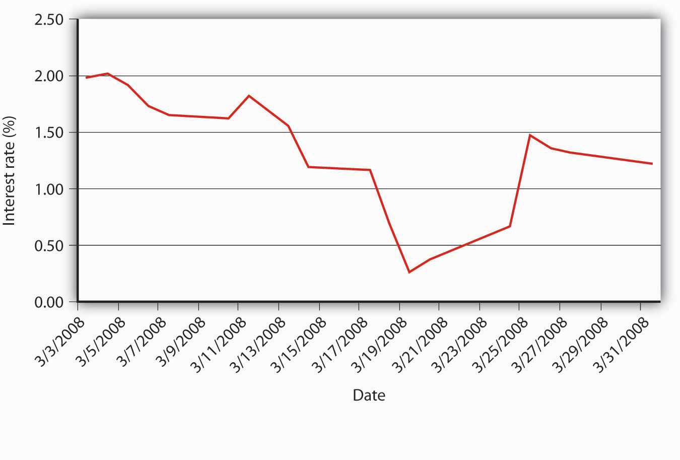
If you followed the gist of Chapter 4 "Interest Rates", you learned (we hope!) about the time value of money, including how to calculate future value (FV), present value (PV), yield to maturity, current yield (the yield to maturity of a perpetuity), rate of return, and real interest rates. You also learned that a change in the interest rate has a profound effect on the value of assets, especially bonds and other types of loans, but also equities and derivatives. (In this chapter, we’ll use the generic term bonds throughout.) That might not be a very important insight if interest rates were stable for long periods. The fact is, however, interest rates change monthly, weekly, daily, and even, in some markets, by the nanosecond. Consider Figure 5.1 "Yields on one-month U.S. Treasury bills, 2001–2008" and Figure 5.2 "Yields on one-month U.S. Treasury bills, March 2008". The first figure shows yields on one-month U.S. Treasury bills from 2001 to 2008, the second shows a zoomed-in view on just March 2008. Clearly, there are long-term secular trends as well as short-term ups and downs.

Figure 5.1 Yields on one-month U.S. Treasury bills, 2001–2008

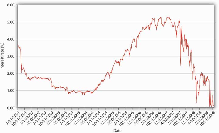
Figure 5.2 Yields on one-month U.S. Treasury bills, March 2008

You should now be primed to ask, Why does the interest rate fluctuate? In other words, What causes interest rate movements like those shown above? In this aptly named chapter, we will examine the economic factors that determine the nominal interest rate. We will ignore, until the next chapter, the fact that interest rates differ on different types of securities. As we’ll learn in Chapter 6 "The Economics of Interest-Rate Spreads and Yield Curves", interest rates tend to track each other, so by focusing on what makes one interest rate move, we have a leg up on making sense of movements in the literally thousands of interest rates out there in the real world. Another way to think about this is that, in this chapter, we will concern ourselves only with the general level of interest rates, which economists call “the” interest rate.

The keys to understanding why “the” interest rate changes over time are simple price theory (supply and demand), the theory of asset demand, and the liquidity preference framework of renowned early twentieth-century British economist John Maynard Keynes.http://www-history.mcs.st-andrews.ac.uk/Biographies/Keynes.html Like other types of goods, bonds and other financial instruments trade in markets. The demand curve for bonds, as for most goods, slopes downward; the supply curve slopes upward in the usual fashion. There is little mystery here. The supply curve slopes upward because, as the price of bonds increases (which is to say, as we learned in Chapter 4 "Interest Rates", as their yield to maturity decreases), ceteris paribus, borrowers (sellers of securities) will supply a higher quantity, just as producers facing higher prices for their wares will supply more cheese or automobiles. As the price of bonds falls, or as the yield to maturity that sellers and borrowers offer increases, sellers and borrowers will supply fewer bonds. (Why sell ’em if they aren’t going to fetch much?) The demand curve for bonds slopes downward for similar reasons. When bond prices are high (yields to maturity are low), few will be demanded. As their price falls (their yields increase), investors (buyers) want more of them because they are increasingly good deals.

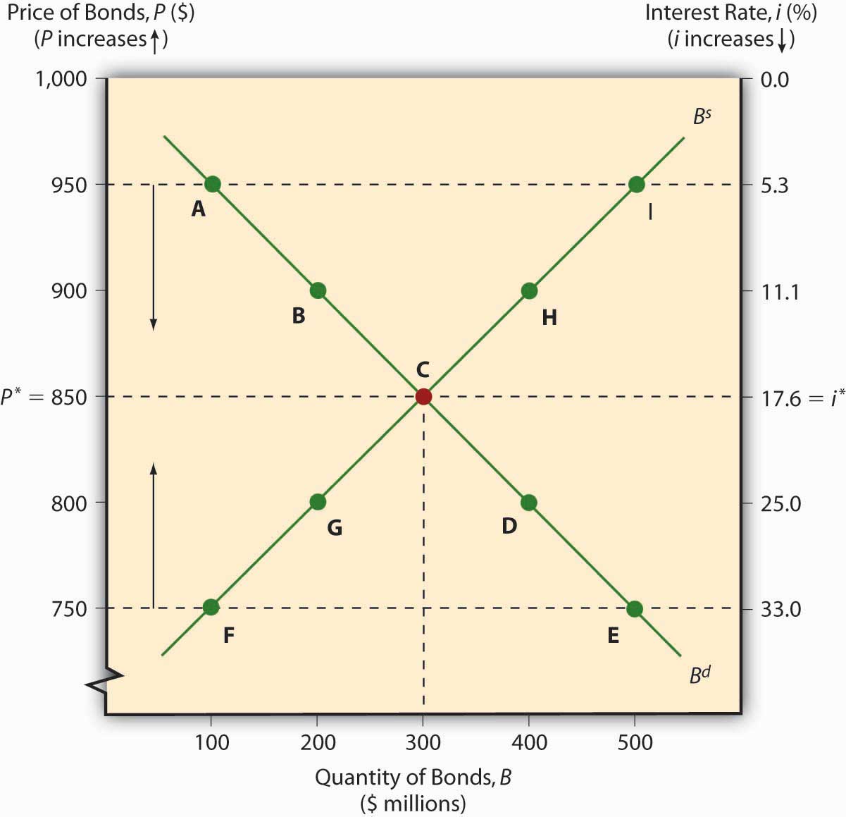
The market price of a bond and the quantity that will be traded is determined, of course, by the intersection of the supply and demand curves, as in Figure 5.3 "Equilibrium in the bond market". The equilibrium price prevails in the market because, if the market price were temporarily greater than p*, the market would be glutted with bonds. In other words, the quantity of bonds supplied would exceed the quantity demanded, so sellers of bonds would lower their asking price until equilibrium was restored. If the market price temporarily dipped below p*, excess demand would prevail (the quantity demanded would exceed the quantity supplied), and investors would bid up the price of the bonds to the equilibrium point.

Figure 5.3 Equilibrium in the bond market

As with other goods, the supply and demand curves for bonds can shift right or left, with results familiar to principles (“Econ 101”) students. If the supply of bonds increases (the supply curve shifts right), the market price will decrease (the interest rate will increase) and the quantity of bonds traded will increase. If the supply of bonds decreases (the supply curve shifts left), bond prices increase (the interest rate falls) and the equilibrium quantity decreases. If the demand for bonds falls (the demand curve shifts left), prices and quantities decrease (and the interest rate increases). If demand increases (the demand curve shifts right), prices and quantities rise (and the interest rate falls).

5.2 Shifts in Supply and Demand for Bonds

Shifting supply and demand curves around can be fun, but figuring out why the curves shift is the interesting part. (Determining the shape and slope of the curves is interesting too, but these details will not detain us here.) Movements along the curve, or why the supply curve slopes upward and the demand curve downward, were easy enough to grasp. Determining why the whole curve moves, why investors are willing to buy more (or fewer) bonds, or why borrowers are willing to sell more (or fewer) bonds at a given price is a bit more involved. Let’s tackle demand first, then we will move on to supply.

Wealth determines the overall demand for assets. An asset (something owned) is any store of value, including financial assets like money, loans (for the lender), bonds, equities (stocks), and a potpourri of derivativeshttp://www.margrabe.com/Dictionary/DictionaryAC.html#sectA and nonfinancial assets like real estate (land, buildings), precious metals (gold, silver, platinum), gems (diamonds, rubies, emeralds), hydrocarbons (oil, natural gas) and (to a greater or lesser extent, depending on their qualities) all other physical goods (as opposed to bads, like pollution, or freebies, like air). As wealth increases, so too does the quantity demanded of all types of assets, though to different degrees. The reasoning here is almost circular: if it is to be maintained, wealth must be invested in some asset, in some store of value. In which type of asset to invest new wealth is the difficult decision. When determining which assets to hold, most economic entities (people, firms, governments) care about many factors, but for most investors most of the time, three variables—expected relative return, risk, and liquidity—are paramount. (We briefly discussed these concepts, you may recall, in Chapter 2 "The Financial System".)

Expected relative return is the ex ante (before the fact) belief that the return on one asset will be higher than the returns of other comparable (in terms of risk and liquidity) assets. Return is a good thing, of course, so as expected relative return increases, the quantity demanded of an asset also increases. That can happen because the expected return on the asset itself increases, because the expected return on comparables decreases, or because of a combination thereof. Clearly, two major factors discussed in Chapter 4 "Interest Rates" will affect return expectations and hence the demand for certain financial assets, like bonds: expected interest rates and, via the Fisher Equation, expected inflation. If the interest rate is expected to increase for any reason (including, but not limited to, expected increases in inflation), bond prices are expected to fall, so the quantity demanded will decrease. Conversely, if the interest rate is thought to decrease for any reason (including, but not limited to, the expected taming of inflation), bond prices are expected to rise, so the quantity demanded will increase.

Overall, though, calculating relative expected returns is sticky business that is best addressed in more specialized financial books and courses. If you want an introduction, investigate the capital asset pricing model (CAPM)http://www.valuebasedmanagement.net/methods_capm.html;http://www.moneychimp.com/articles/valuation/capm.htm and the arbitrage pricing theory (APT).http://moneyterms.co.uk/apt/ As we learned in Chapter 4 "Interest Rates", calculating return is not terribly difficult and neither is comparing returns among a variety of assets. What’s tricky is forecasting future returns and making sure that assets are comparable by controlling for risk, among other things. Risk is the uncertainty of an asset’s returns. It comes in a variety of flavors, all of them unsavory, so as it increases, the quantity demanded of an asset decreases, ceteris paribus. In Chapter 4 "Interest Rates", we encountered two types of risk: default risk (aka credit risk), the chance that a financial contract will not be honored, and interest rate risk, the chance that the interest rate will rise and hence decrease a bond or loan’s price. An offsetting risk is called reinvestment risk, which bites when the interest rate decreases because coupon or other interest payments have to be reinvested at a lower yield to maturity. To be willing to take on more risk, whatever its flavor, rational investors must expect a higher relative return. Investors who require a much higher return for assuming a little bit of risk are called risk-averse. Those who will take on much risk for a little higher return are called risk-loving, risk-seekers, or risk-tolerant. (Investors who take on more risk without compensation are neither risk-averse nor risk-tolerant, but rather irrational in the sense discussed in Chapter 7 "Rational Expectations, Efficient Markets, and the Valuation of Corporate Equities".) Risks can be idiosyncratic; that is, they can be pertinent to a particular company, sectoral (pertinent to an entire industry, like trucking or restaurants), or systemic (economy-wide). Liquidity risk occurs when an asset cannot be sold as quickly or cheaply as expected, be it for idiosyncratic, sectoral, or systemic reasons. This, too, is a serious risk because liquidity, or (to be more precise) liquidity relative to other assets, is the third major determinant of asset demand. Because investors often need to change their investment portfolioThe set of financial and other investments or assets held by an economic entity. or dis-save (spend some of their wealth on consumption), liquidity, the ability to sell an asset quickly and cheaply, is a good thing. The more liquid an asset is, therefore, the higher the quantity demanded, all else being equal.

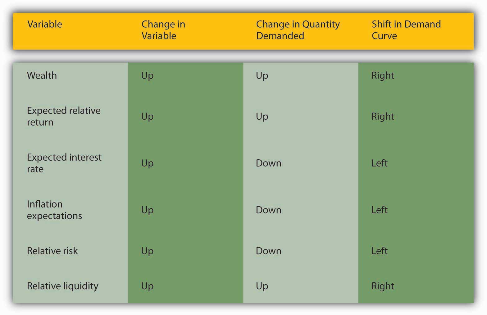
During the financial crisis that began in 2007, the prices of a certain type of bond collateralized by subprime mortgages, long-term loans collateralized with homes and made to relatively risky borrowers, collapsed. In other words, their yields had to increase markedly to induce investors to own them. They dropped in price after investors realized that the bonds, a type of asset-backed security (ABS), had much higher default rates and much lower levels of liquidity than they had previously believed. Figure 5.4 "Variables that influence demand for bonds" summarizes the chapter discussion so far.

Figure 5.4 Variables that influence demand for bonds

So much for demand. Why does the supply curve for bonds shift to and fro? There are many reasons, but the three main ones are government budgets, inflation expectations, and general business conditions. When governments run budget deficits, they often borrow by selling bonds, pushing the supply curve rightward and bond prices down (yields up), ceteris paribus. When governments run surpluses, and they occasionally do, believe it or not, they redeem and/or buy their bonds back on net, pushing the supply curve to the left and bond prices up (yields down), all else being equal. (For historical time series data on the U.S. national debt, which was usually composed mostly of bonds, browse http://www.economagic.com/em-cgi/data.exe/treas/pubdebt.)

The expectation of higher inflation, other factors held constant, will cause borrowers to issue more bonds, driving the supply curve rightward, and bond prices down (and yields up). The Fisher Equation, i_r = i – π^e, explains this nicely. If the inflation expectation term π^e increases while nominal interest rate i stays the same, the real interest rate i_r must decrease. From the perspective of borrowers, the real cost of borrowing falls, which means that borrowing becomes more attractive. So they sell bonds.

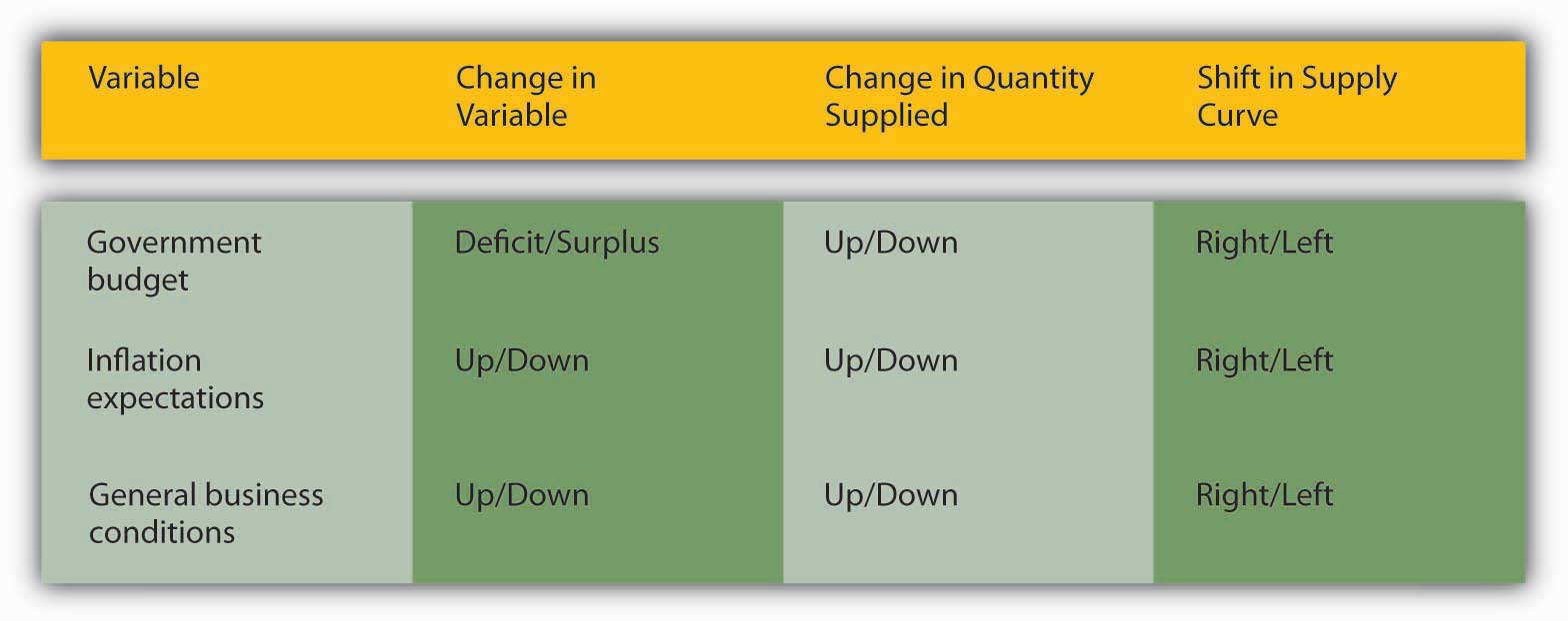
Borrowing also becomes more attractive when general business conditions become more favorable, as when taxes and regulatory costs decrease or the economy expands. Although individuals sometimes try to borrow out of financial weakness or desperation, relatively few such loans are made because they are high risk. Most economic entities borrow out of strength, to finance expansion and engage in new projects they believe will be profitable. So when economic prospects are good, taxes are low, and regulations are not too costly, businesses are eager to borrow, often by selling bonds, shifting the supply curve to the right and bond prices down (yields up). Figure 5.5 "Variables that determine the supply of bonds" summarizes the chapter discussion so far.

Figure 5.5 Variables that determine the supply of bonds

As Yoda might say, “Pause here, we must” to make sure we’re on track.http://www.yodaspeak.co.uk/index.php Try out these questions until you are comfortable. Remember that the ceteris paribus condition holds in each.

Exercises

1. What will happen to bond prices if stock trading commissions decrease? Why?
2. What will happen to bond prices if bond trading commissions increase? Why?
3. What will happen to bond prices if the government implements tax increases? Why?
4. If government revenues drop significantly (and remember all else stays the same, including government expenditures), what will likely happen to bond prices? Why?
5. If the government guaranteed the payment of bonds, what would happen to their prices? Why?
6. What will happen to bond prices if the government implements regulatory reforms that reduce regulatory costs for businesses? Why?
7. If government revenues increase significantly, what will likely happen to bond prices? Why?
8. What will happen to bond prices if terrorism ended and the world’s nations unilaterally disarmed and adopted free trade policies? Why?
9. What will happen to bond prices if world peace brought substantially lower government budget deficits?

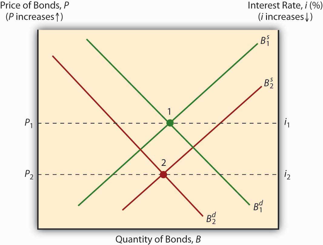
If you’ve already figured out that expected inflation will decrease bond prices, and increase bond yields, by both shifting the supply curve to the right and the demand curve to the left, as in Figure 5.6 "Expected inflation and bond prices" below, kudos to you!

Figure 5.6 Expected inflation and bond prices

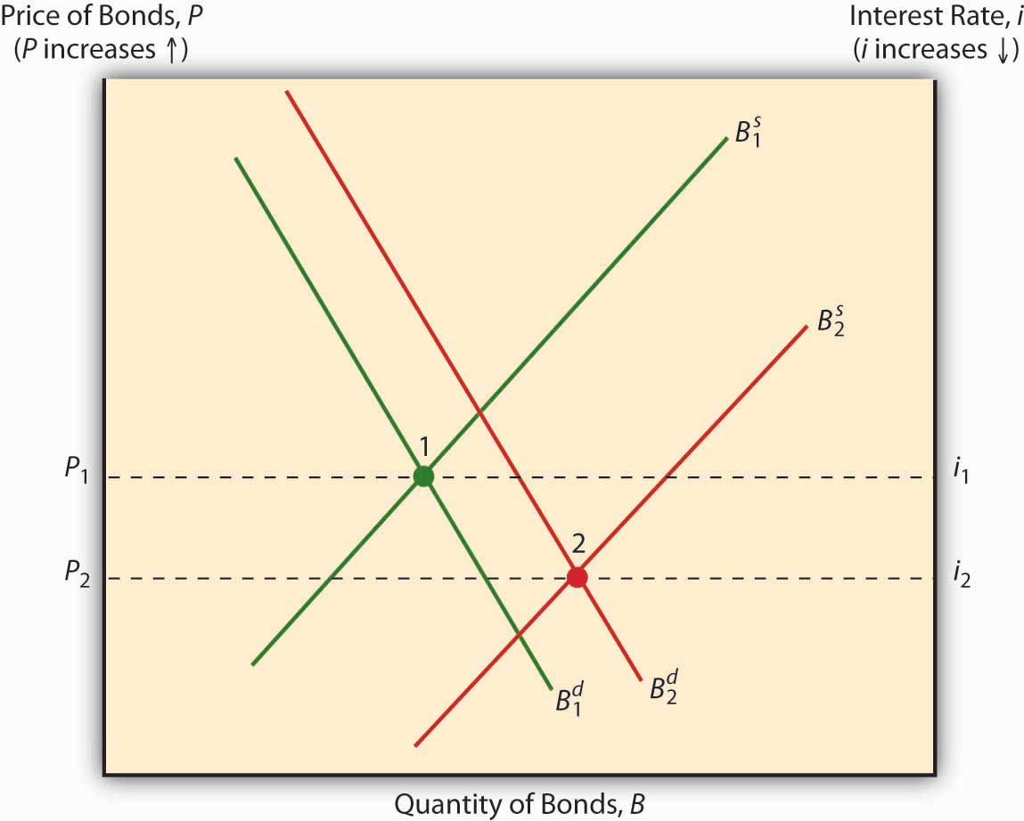
If you noticed that the response of bond prices and yields to a business cycle expansion is indeterminate, booya! As noted above, a boom shifts the bond supply curve to the right by inducing businesses to borrow and thus take advantage of the bonanza. Holding demand constant, that action reduces bond prices (raises the interest rate). But demand does not stay constant because economic expansion increases wealth, which increases demand for bonds (shifts the curve to the right), which in turn increases bond prices (reduces the interest rate). The net effect on the interest rate, therefore, depends on how much each curve shifts, as in Figure 5.7 "Business cycle expansion and bond prices".

Figure 5.7 Business cycle expansion and bond prices

In reality, the first scenario is the one that usually wins out: during expansions, the interest rate usually rises, and during recessions, it always falls. For example, the interest rate fell to very low levels during the Great DepressionAn almost worldwide decrease in per capita income during the 1930s. and during Japan’s extended economic funkFunk is not a technical term, but it is used widely because it encapsulates the economic situation in Japan in a single interesting word. After World War II, Japan experienced rapid economic growth. That growth slowed considerably in the 1990s, following a major financial crisis. in the 1990s.http://www.bloomberg.com/apps/news?pid=10000101&refer=japan&sid=a28sELjm9W04

5.3 Liquidity Preference

Elementary price theory and the theory of asset demand go a long way toward helping us to understand why the interest rate bobbles up and down over time. A third aid to our understanding, the liquidity preference framework, strengthens our conviction in the robustness of our analyses and adds nuance to our understanding. In this model there are but two assets, money, which earns no interest, and bonds, which earn some interest greater than zero. (The two-asset assumption needn’t worry you. Economic models deliberately simplify reality to concentrate on what is most important.http://en.wikipedia.org/wiki/Model_(economics)) Furthermore, in the model, the markets for bonds and money are both in equilibrium, so we can study the latter to learn about the former.

Graphically, the model is most easily represented as shown in Figure 5.8 "Equilibrium in the market for money". It is a little different than what you are used to because the vertical axis is the interest rate, not price. Other than that, the graph works exactly like a traditional supply and demand graph. The money demand curve slopes downward in the usual way because, as the interest rate increases, the quantity of money demanded decreases. Why hoard cash when you can buy bonds with it and make beaucoup bucks? As the interest rate declines, though, the quantity of money demanded will increase as the opportunity cost of holding bonds decreases. Why own bonds, which of course aren’t as liquid as money, if they pay squat? The supply of money in this model is represented by a vertical line. It can slide left and right if the monetary authority (like a government central bank, of which you will learn more in Chapter 13 "Central Bank Form and Function") sees fit to decrease or increase the money supply, respectively, but the quantity supplied does not vary with changes in the interest rate. (In more technical parlance, the supply of money in the model is perfectly inelastic.)

Figure 5.8 Equilibrium in the market for money

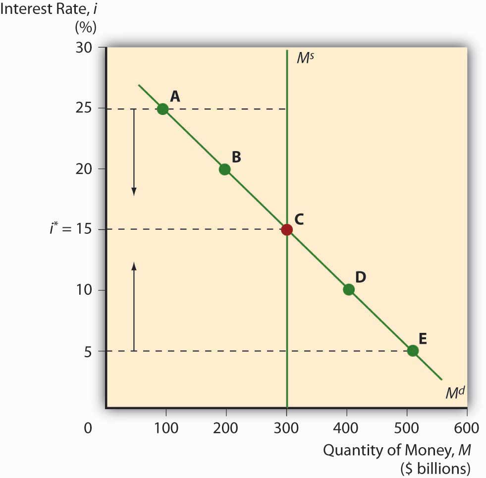
The intersection of the money supply and demand curves reveals the market rate of interest. Equilibrium will be reached because, if the interest rate exceeds the equilibrium rate (i*), the quantity of money demanded will be less than the quantity of money supplied. People will use their excess money to buy bonds, which will drive bond prices up and yields down, toward the equilibrium. Conversely, if the interest rate is below the equilibrium rate, the quantity of money demanded exceeds the quantity supplied. People would therefore sell bonds for cash, decreasing bond prices and increasing bond yields until the equilibrium is reached.

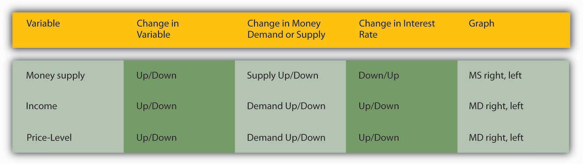
The equilibrium interest rate i* changes, of course, with movements of either curve. If the money supply increases (the money supply curve shifts right), the interest rate falls, ceteris paribus. That makes sense because there is more money to lend. If the money supply decreases, by contrast, the interest rate increases because there is less money to lend (and the demand stays the same). The demand for money can also change. If the demand curve shifts right (and the money supply stays constant), higher demand for money will spell a higher interest rate. If it shifts left, lower money demand will cause the interest rate to decrease. Again, this makes great sense intuitively.

The interesting issue here is why the curves move, not what happens when they do. According to the model, the money demand curve shifts for two major reasons, income and price level, both of which are positively related to demand. In other words, as income increases or the price level rises, the demand for money increases (shifting the money demand curve to the right and thus increasing the interest rate). Money demand increases with income for two reasons: because money is an asset and hence demand for it increases with wealth, as described above. Perhaps more important, money demand increases because economic entities transact more as incomes rise, so they need more money to make payments. Inflation increases money demand because people care about real balances, not nominal ones. As the price level rises, the same sum of money cannot buy as much, so people demand more money at any given interest rate (i.e., the money demand curve shifts right) and, in accord with the Fisher Equation, the interest rate rises.

Figure 5.9 "Determinants of the supply and demand for money" summarizes the chapter discussion so far. And it’s time again to complete some problems and make sure you’re following all this.

Figure 5.9 Determinants of the supply and demand for money

5.4 Predictions and Effects

We’re almost there! As noted above, the liquidity preference framework predicts that increasing the money supply will decrease the interest rate. This liquidity effect, as it is called, holds if all other factors, including income, actual inflation, and expected inflation, remain the same. In the distant past, the ceteris paribus condition indeed held, as suggested in Figure 5.10 "United States financial money meter, ca. 1800". The excerpt in the figure is taken from an early nineteenth-century economic treatise.

Figure 5.10 United States financial money meter, ca. 1800

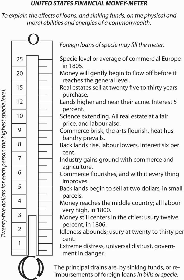
The key point is that, as the money supply (here presented in per capita terms, from $1 to $25 per person) increases, the interest rate falls, as the model predicts. At $2 per person “usury,” an antiquated term for “interest,” is at “twenty to thirty percent.” At $3, it falls to 12 percent, as in 1806. At $8 per head, it sinks to 6 percent, while at $12, it goes to 5, and at $15, to 3.33 or 4. (“Real estates sell at twenty five to thirty years purchase” is an old-fashioned way of stating this. Think about it in terms of the perpetuity equation you learned in Chapter 4 "Interest Rates": i = FV/PV, where FV is 1 and PV 25 or 30 times that, 25 or 30 times the annual income generated by the asset. i = 1/25 = .04 and i = 1/30 = .033333.) Most of the world was on a commodity standard (gold and/or silver) then, so the money supply was self-equilibrating, expanding and contracting automatically, as explained in Chapter 3 "Money". At $20 or so per person, money began to “flow off,” i.e., to be exported, and would never exceed $25. So monetary expansion did not cause prices to rise permanently; the expectation was one of zero net inflation in the medium to long term.

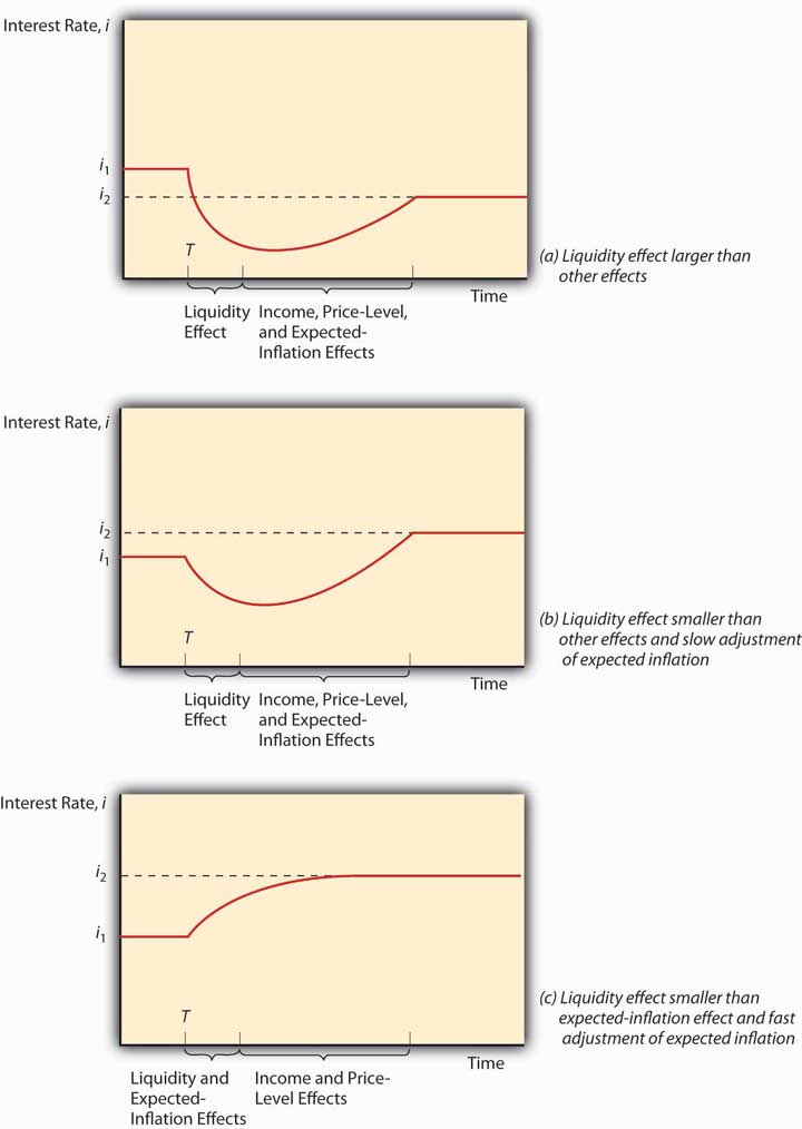
Today, matters are rather different. Government entities regulate the money supply and have a habit of expanding it because doing so prudently increases economic growth, employment, incomes, and other good stuff. Unfortunately, expanding the money supply also causes prices to rise almost every year, with no reversion to earlier levels. When the money supply increases today, therefore, inflation often actually occurs and people begin to expect inflation in its wake. Each of these three effects, called the income, price level, and expected inflation effects, causes the interest rate to rise for the reasons discussed above. When the money supply increases, the liquidity effect, which lowers the interest rate, battles these three countervailing effects. Sometimes, as in the distant past, the liquidity effect wins out. When the money supply increases (or increases faster than usual), the liquidity effect wins out, and the interest rate declines and stays below the previous level. Sometimes, often in modern industrial economies with independent central banksA monetary authority that is controlled by public-interested technocrats rather than by self-interested politicians. For more information, see Chapter 13 "Central Bank Form and Function"., the liquidity effect wins at first and the interest rate declines, but then incomes rise, inflation expectations increase, and the price level actually rises, eventually causing the interest rate to increase above the original level. Finally, sometimes, as in modern undeveloped countries with weak central banking institutions, the expectation of inflation is so strong and so quick that it overwhelms the liquidity effect, driving up the interest rate immediately. Later, after incomes and the price level increase, the interest rate soars yet higher. Figure 5.11 "Money supply growth and nominal interest rates" summarizes this discussion graphically.

Figure 5.11 Money supply growth and nominal interest rates

The ability to forecast changes in the interest rate is a rare but profitable gift. Professional interest rate forecasters are rarely right on the mark and often are far astray,www.finpipe.com/intratgo.htm and half the time they don’t even get the direction (up or down) right.taylorandfrancis.metapress.com/(vqspd445seikpajibz05ch45)/app/home/contribution.asp?referrer =parent&backto=issue,5,9;journal,15,86;linkingpublicationresults,1:100411,1 That’s what we’d expect if their forecasts were determined by flipping a coin! We’ll discuss why this might be in Chapter 7 "Rational Expectations, Efficient Markets, and the Valuation of Corporate Equities". Therefore, we don’t expect you to be able to predict changes in the interest rate, but we do expect you to be able to post-dict them. In other words, you should be able to narrate, in words and appropriate graphs, why past changes occurred. You should also be able to make predictions by invoking the ceteris paribus assumption.

5.5 Suggested Reading

Bibow, Jorg. Keynes on Monetary Policy, Finance and Uncertainty: Reassessing Liquidity Preference Theory. New York: Routledge, 2009.

Evans, Michael. Practical Business Forecasting. Hoboken, NJ: John Wiley and Sons, 2002.

Friedman, Milton. The Optimum Quantity of Money. Piscataway, NJ: Aldine Transaction, 2005.