This is “Modelling Linear Relationships with Randomness Present”, section 10.3 from the book Beginning Statistics (v. 1.0). For details on it (including licensing), click here.
For more information on the source of this book, or why it is available for free, please see the project's home page. You can browse or download additional books there. To download a .zip file containing this book to use offline, simply click here.


10.3 Modelling Linear Relationships with Randomness Present
Learning Objective
- To learn the framework in which the statistical analysis of the linear relationship between two variables x and y will be done.
In this chapter we are dealing with a population for which we can associate to each element two measurements, x and y. We are interested in situations in which the value of x can be used to draw conclusions about the value of y, such as predicting the resale value y of a residential house based on its size x. Since the relationship between x and y is not deterministic, statistical procedures must be applied. For any statistical procedures, given in this book or elsewhere, the associated formulas are valid only under specific assumptions. The set of assumptions in simple linear regression are a mathematical description of the relationship between x and y. Such a set of assumptions is known as a model.
For each fixed value of x a sub-population of the full population is determined, such as the collection of all houses with 2,100 square feet of living space. For each element of that sub-population there is a measurement y, such as the value of any 2,100-square-foot house. Let denote the mean of all the y-values for each particular value of x. can change from x-value to x-value, such as the mean value of all 2,100-square-foot houses, the (different) mean value for all 2,500-square foot-houses, and so on.
Our first assumption is that the relationship between x and the mean of the y-values in the sub-population determined by x is linear. This means that there exist numbers and such that
This linear relationship is the reason for the word “linear” in “simple linear regression” below. (The word “simple” means that y depends on only one other variable and not two or more.)
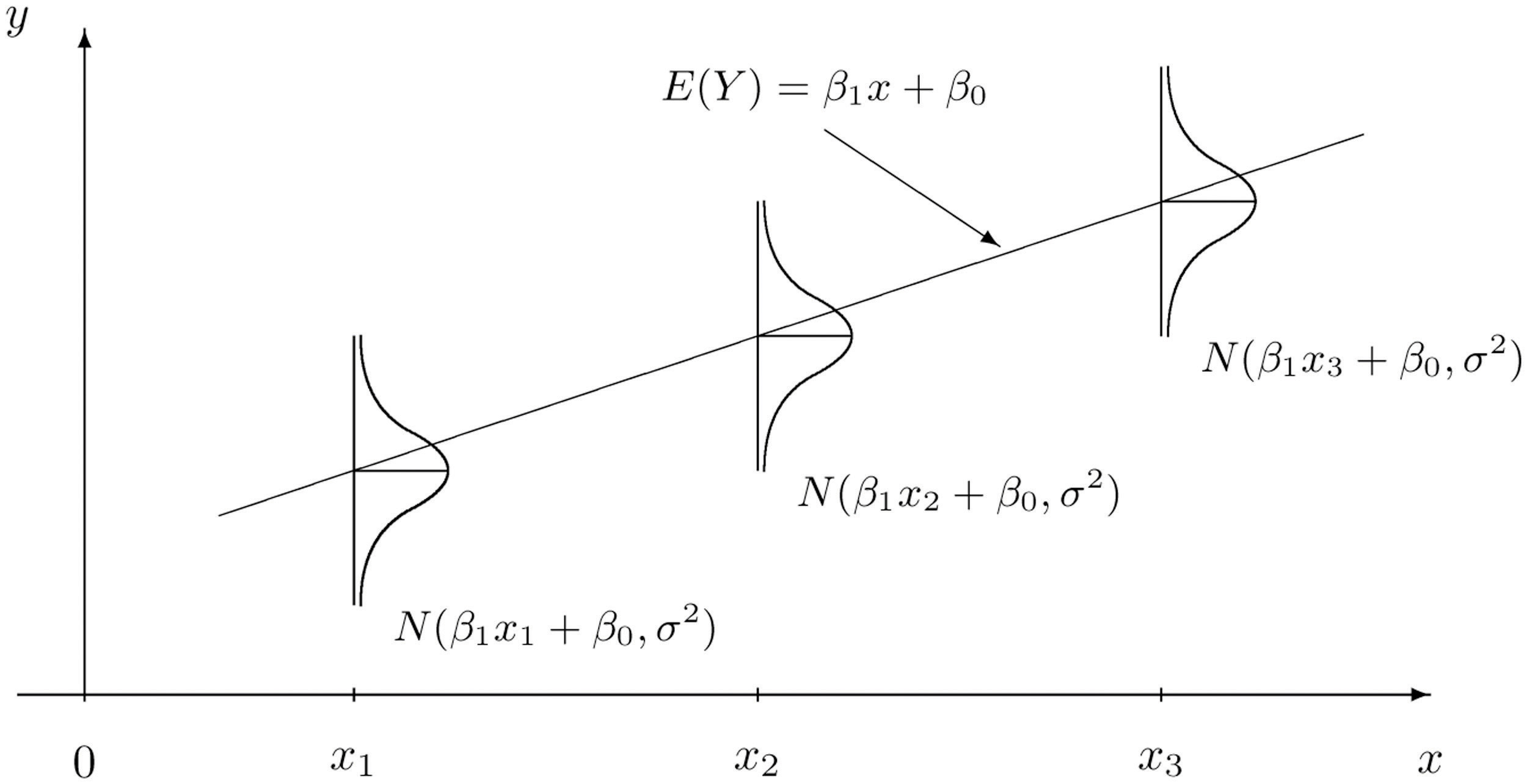
Our next assumption is that for each value of x the y-values scatter about the mean according to a normal distribution centered at and with a standard deviation σ that is the same for every value of x. This is the same as saying that there exists a normally distributed random variable ε with mean 0 and standard deviation σ so that the relationship between x and y in the whole population is
Our last assumption is that the random deviations associated with different observations are independent.
In summary, the model is:
Simple Linear Regression Model
For each point in data set the y-value is an independent observation of
where and are fixed parameters and ε is a normally distributed random variable with mean 0 and an unknown standard deviation σ.
The line with equation is called the population regression lineThe line with equation that gives the mean of the variable y over the sub-population determined by x..
Figure 10.5 "The Simple Linear Model Concept" illustrates the model. The symbols denote a normal distribution with mean μ and variance , hence standard deviation σ.
Figure 10.5 The Simple Linear Model Concept
It is conceptually important to view the model as a sum of two parts:
- Deterministic Part. The first part is the equation that describes the trend in y as x increases. The line that we seem to see when we look at the scatter diagram is an approximation of the line There is nothing random in this part, and therefore it is called the deterministic part of the model.
- Random Part. The second part ε is a random variable, often called the error term or the noise. This part explains why the actual observed values of y are not exactly on but fluctuate near a line. Information about this term is important since only when one knows how much noise there is in the data can one know how trustworthy the detected trend is.
There are three parameters in this model: , , and σ. Each has an important interpretation, particularly and σ. The slope parameter represents the expected change in y brought about by a unit increase in x. The standard deviation σ represents the magnitude of the noise in the data.
There are procedures for checking the validity of the three assumptions, but for us it will be sufficient to visually verify the linear trend in the data. If the data set is large then the points in the scatter diagram will form a band about an apparent straight line. The normality of ε with a constant standard deviation corresponds graphically to the band being of roughly constant width, and with most points concentrated near the middle of the band.
Fortunately, the three assumptions do not need to hold exactly in order for the procedures and analysis developed in this chapter to be useful.
Key Takeaway
- Statistical procedures are valid only when certain assumptions are valid. The assumptions underlying the analyses done in this chapter are graphically summarized in Figure 10.5 "The Simple Linear Model Concept".
Exercises
-
State the three assumptions that are the basis for the Simple Linear Regression Model.
-
The Simple Linear Regression Model is summarized by the equation
Identify the deterministic part and the random part.
-
Is the number in the equation a statistic or a population parameter? Explain.
-
Is the number σ in the Simple Linear Regression Model a statistic or a population parameter? Explain.
-
Describe what to look for in a scatter diagram in order to check that the assumptions of the Simple Linear Regression Model are true.
-
True or false: the assumptions of the Simple Linear Regression Model must hold exactly in order for the procedures and analysis developed in this chapter to be useful.
Answers
-
- The mean of y is linearly related to x.
- For each given x, y is a normal random variable with mean and standard deviation σ.
- All the observations of y in the sample are independent.
-
-
is a population parameter.
-
-
A linear trend.
-