This is “Linear Relationships Between Variables”, section 10.1 from the book Beginning Statistics (v. 1.0). For details on it (including licensing), click here.
For more information on the source of this book, or why it is available for free, please see the project's home page. You can browse or download additional books there. To download a .zip file containing this book to use offline, simply click here.


10.1 Linear Relationships Between Variables
Learning Objective
- To learn what it means for two variables to exhibit a relationship that is close to linear but which contains an element of randomness.
The following table gives examples of the kinds of pairs of variables which could be of interest from a statistical point of view.
| x | y |
|---|---|
| Predictor or independent variable | Response or dependent variable |
| Temperature in degrees Celsius | Temperature in degrees Fahrenheit |
| Area of a house (sq.ft.) | Value of the house |
| Age of a particular make and model car | Resale value of the car |
| Amount spent by a business on advertising in a year | Revenue received that year |
| Height of a 25-year-old man | Weight of the man |
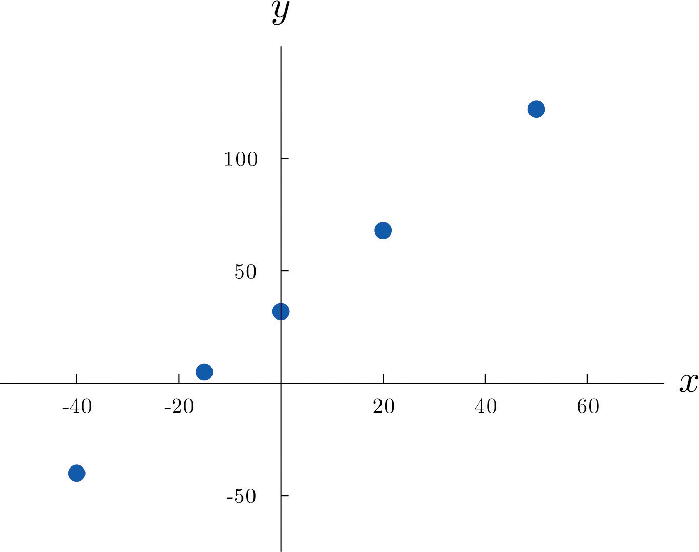
The first line in the table is different from all the rest because in that case and no other the relationship between the variables is deterministic: once the value of x is known the value of y is completely determined. In fact there is a formula for y in terms of x: Choosing several values for x and computing the corresponding value for y for each one using the formula gives the table
We can plot these data by choosing a pair of perpendicular lines in the plane, called the coordinate axes, as shown in Figure 10.1 "Plot of Celsius and Fahrenheit Temperature Pairs". Then to each pair of numbers in the table we associate a unique point in the plane, the point that lies x units to the right of the vertical axis (to the left if ) and y units above the horizontal axis (below if ). The relationship between x and y is called a linear relationship because the points so plotted all lie on a single straight line. The number in the equation is the slope of the line, and measures its steepness. It describes how y changes in response to a change in x: if x increases by 1 unit then y increases (since is positive) by unit. If the slope had been negative then y would have decreased in response to an increase in x. The number 32 in the formula is the y-intercept of the line; it identifies where the line crosses the y-axis. You may recall from an earlier course that every non-vertical line in the plane is described by an equation of the form , where m is the slope of the line and b is its y-intercept.
Figure 10.1 Plot of Celsius and Fahrenheit Temperature Pairs
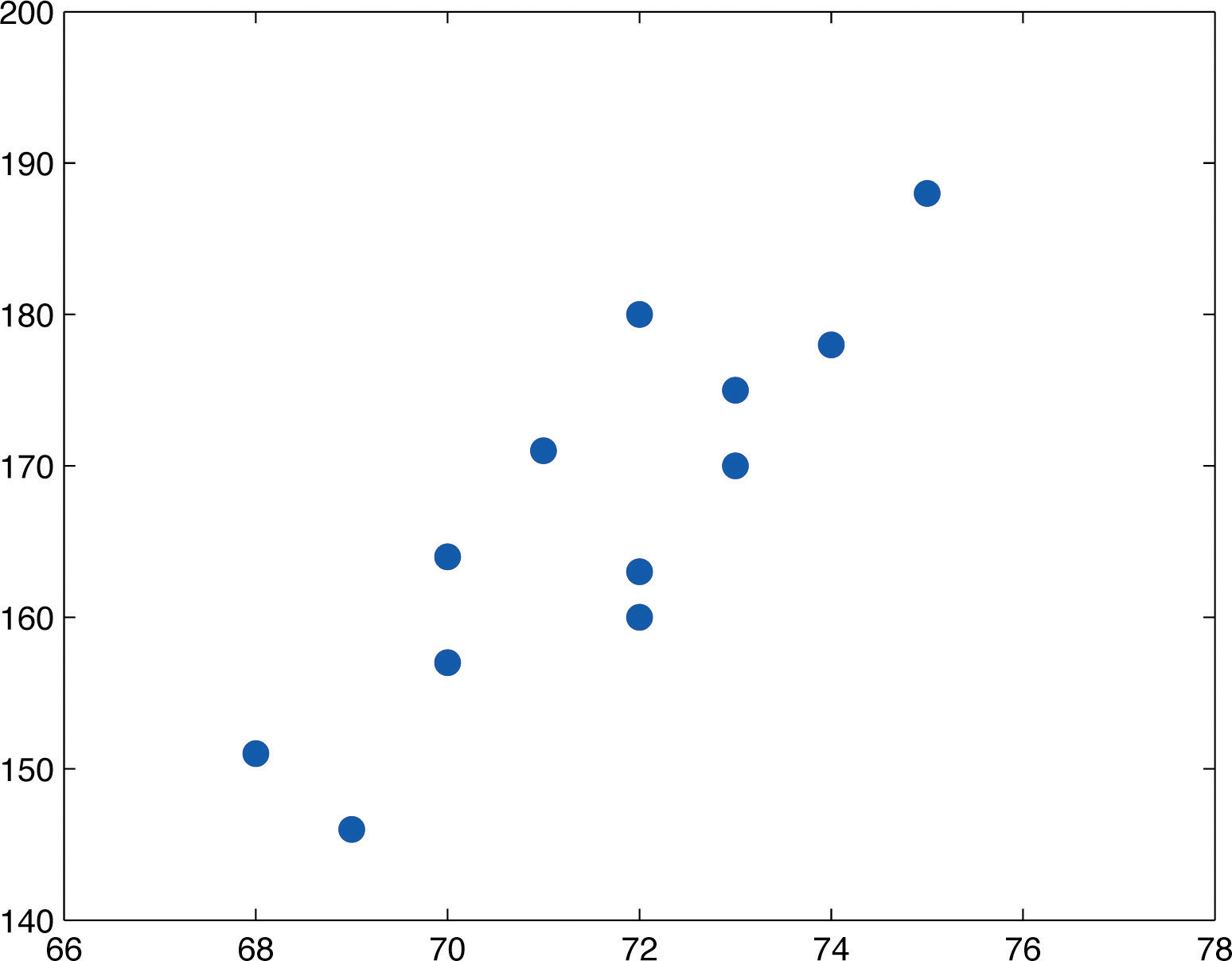
The relationship between x and y in the temperature example is deterministic because once the value of x is known, the value of y is completely determined. In contrast, all the other relationships listed in the table above have an element of randomness in them. Consider the relationship described in the last line of the table, the height x of a man aged 25 and his weight y. If we were to randomly select several 25-year-old men and measure the height and weight of each one, we might obtain a collection of pairs something like this:
A plot of these data is shown in Figure 10.2 "Plot of Height and Weight Pairs". Such a plot is called a scatter diagram or scatter plot. Looking at the plot it is evident that there exists a linear relationship between height x and weight y, but not a perfect one. The points appear to be following a line, but not exactly. There is an element of randomness present.
Figure 10.2 Plot of Height and Weight Pairs
In this chapter we will analyze situations in which variables x and y exhibit such a linear relationship with randomness. The level of randomness will vary from situation to situation. In the introductory example connecting an electric current and the level of carbon monoxide in air, the relationship is almost perfect. In other situations, such as the height and weights of individuals, the connection between the two variables involves a high degree of randomness. In the next section we will see how to quantify the strength of the linear relationship between two variables.
Key Takeaways
- Two variables x and y have a deterministic linear relationship if points plotted from pairs lie exactly along a single straight line.
- In practice it is common for two variables to exhibit a relationship that is close to linear but which contains an element, possibly large, of randomness.
Exercises
-
A line has equation
- Pick five distinct x-values, use the equation to compute the corresponding y-values, and plot the five points obtained.
- Give the value of the slope of the line; give the value of the y-intercept.
-
A line has equation
- Pick five distinct x-values, use the equation to compute the corresponding y-values, and plot the five points obtained.
- Give the value of the slope of the line; give the value of the y-intercept.
-
A line has equation
- Pick five distinct x-values, use the equation to compute the corresponding y-values, and plot the five points obtained.
- Give the value of the slope of the line; give the value of the y-intercept.
-
A line has equation
- Pick five distinct x-values, use the equation to compute the corresponding y-values, and plot the five points obtained.
- Give the value of the slope of the line; give the value of the y-intercept.
-
Based on the information given about a line, determine how y will change (increase, decrease, or stay the same) when x is increased, and explain. In some cases it might be impossible to tell from the information given.
- The slope is positive.
- The y-intercept is positive.
- The slope is zero.
-
Based on the information given about a line, determine how y will change (increase, decrease, or stay the same) when x is increased, and explain. In some cases it might be impossible to tell from the information given.
- The y-intercept is negative.
- The y-intercept is zero.
- The slope is negative.
-
A data set consists of eight pairs of numbers:
- Plot the data in a scatter diagram.
- Based on the plot, explain whether the relationship between x and y appears to be deterministic or to involve randomness.
- Based on the plot, explain whether the relationship between x and y appears to be linear or not linear.
-
A data set consists of ten pairs of numbers:
- Plot the data in a scatter diagram.
- Based on the plot, explain whether the relationship between x and y appears to be deterministic or to involve randomness.
- Based on the plot, explain whether the relationship between x and y appears to be linear or not linear.
-
A data set consists of nine pairs of numbers:
- Plot the data in a scatter diagram.
- Based on the plot, explain whether the relationship between x and y appears to be deterministic or to involve randomness.
- Based on the plot, explain whether the relationship between x and y appears to be linear or not linear.
-
A data set consists of five pairs of numbers:
- Plot the data in a scatter diagram.
- Based on the plot, explain whether the relationship between x and y appears to be deterministic or to involve randomness.
- Based on the plot, explain whether the relationship between x and y appears to be linear or not linear.
Basic
-
At 60°F a particular blend of automotive gasoline weights 6.17 lb/gal. The weight y of gasoline on a tank truck that is loaded with x gallons of gasoline is given by the linear equation
- Explain whether the relationship between the weight y and the amount x of gasoline is deterministic or contains an element of randomness.
- Predict the weight of gasoline on a tank truck that has just been loaded with 6,750 gallons of gasoline.
-
The rate for renting a motor scooter for one day at a beach resort area is $25 plus 30 cents for each mile the scooter is driven. The total cost y in dollars for renting a scooter and driving it x miles is
- Explain whether the relationship between the cost y of renting the scooter for a day and the distance x that the scooter is driven that day is deterministic or contains an element of randomness.
- A person intends to rent a scooter one day for a trip to an attraction 17 miles away. Assuming that the total distance the scooter is driven is 34 miles, predict the cost of the rental.
-
The pricing schedule for labor on a service call by an elevator repair company is $150 plus $50 per hour on site.
- Write down the linear equation that relates the labor cost y to the number of hours x that the repairman is on site.
- Calculate the labor cost for a service call that lasts 2.5 hours.
-
The cost of a telephone call made through a leased line service is 2.5 cents per minute.
- Write down the linear equation that relates the cost y (in cents) of a call to its length x.
- Calculate the cost of a call that lasts 23 minutes.
Applications
-
Large Data Set 1 lists the SAT scores and GPAs of 1,000 students. Plot the scatter diagram with SAT score as the independent variable (x) and GPA as the dependent variable (y). Comment on the appearance and strength of any linear trend.
-
Large Data Set 12 lists the golf scores on one round of golf for 75 golfers first using their own original clubs, then using clubs of a new, experimental design (after two months of familiarization with the new clubs). Plot the scatter diagram with golf score using the original clubs as the independent variable (x) and golf score using the new clubs as the dependent variable (y). Comment on the appearance and strength of any linear trend.
http://www.flatworldknowledge.com/sites/all/files/data12.xls
-
Large Data Set 13 records the number of bidders and sales price of a particular type of antique grandfather clock at 60 auctions. Plot the scatter diagram with the number of bidders at the auction as the independent variable (x) and the sales price as the dependent variable (y). Comment on the appearance and strength of any linear trend.
http://www.flatworldknowledge.com/sites/all/files/data13.xls
Large Data Set Exercises
Answers
-
- Answers vary.
- Slope ; y-intercept
-
-
- Answers vary.
- Slope ; y-intercept
-
-
- y increases.
- Impossible to tell.
- y does not change.
-
-
- Scatter diagram needed.
- Involves randomness.
- Linear.
-
-
- Scatter diagram needed.
- Deterministic.
- Not linear.
-
-
- Deterministic.
- 41,647.5 pounds.
-
-
- b. $275.
-
-
There appears to a hint of some positive correlation.
-
-
There appears to be clear positive correlation.