This is “The Sample Proportion”, section 6.3 from the book Beginning Statistics (v. 1.0). For details on it (including licensing), click here.
For more information on the source of this book, or why it is available for free, please see the project's home page. You can browse or download additional books there. To download a .zip file containing this book to use offline, simply click here.


6.3 The Sample Proportion
Learning Objectives
- To recognize that the sample proportion is a random variable.
- To understand the meaning of the formulas for the mean and standard deviation of the sample proportion.
- To learn what the sampling distribution of is when the sample size is large.
Often sampling is done in order to estimate the proportion of a population that has a specific characteristic, such as the proportion of all items coming off an assembly line that are defective or the proportion of all people entering a retail store who make a purchase before leaving. The population proportion is denoted p and the sample proportion is denoted Thus if in reality 43% of people entering a store make a purchase before leaving, p = 0.43; if in a sample of 200 people entering the store, 78 make a purchase,
The sample proportion is a random variable: it varies from sample to sample in a way that cannot be predicted with certainty. Viewed as a random variable it will be written It has a meanThe number about which proportions computed from samples of the same size center. and a standard deviationA measure of the variability of proportions computed from samples of the same size. Here are formulas for their values.
Suppose random samples of size n are drawn from a population in which the proportion with a characteristic of interest is p. The mean and standard deviation of the sample proportion satisfy
where
The Central Limit Theorem has an analogue for the population proportion To see how, imagine that every element of the population that has the characteristic of interest is labeled with a 1, and that every element that does not is labeled with a 0. This gives a numerical population consisting entirely of zeros and ones. Clearly the proportion of the population with the special characteristic is the proportion of the numerical population that are ones; in symbols,
But of course the sum of all the zeros and ones is simply the number of ones, so the mean μ of the numerical population is
Thus the population proportion p is the same as the mean μ of the corresponding population of zeros and ones. In the same way the sample proportion is the same as the sample mean Thus the Central Limit Theorem applies to However, the condition that the sample be large is a little more complicated than just being of size at least 30.
The Sampling Distribution of the Sample Proportion
For large samples, the sample proportion is approximately normally distributed, with mean and standard deviation
A sample is large if the interval lies wholly within the interval
In actual practice p is not known, hence neither is In that case in order to check that the sample is sufficiently large we substitute the known quantity for p. This means checking that the interval
lies wholly within the interval This is illustrated in the examples.
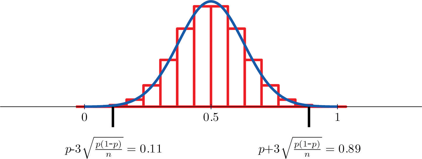
Figure 6.5 "Distribution of Sample Proportions" shows that when p = 0.1 a sample of size 15 is too small but a sample of size 100 is acceptable. Figure 6.6 "Distribution of Sample Proportions for " shows that when p = 0.5 a sample of size 15 is acceptable.
Figure 6.5 Distribution of Sample Proportions
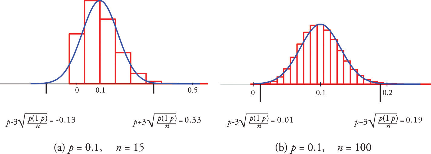
Figure 6.6 Distribution of Sample Proportions for p = 0.5 and n = 15
Example 7
Suppose that in a population of voters in a certain region 38% are in favor of particular bond issue. Nine hundred randomly selected voters are asked if they favor the bond issue.
- Verify that the sample proportion computed from samples of size 900 meets the condition that its sampling distribution be approximately normal.
- Find the probability that the sample proportion computed from a sample of size 900 will be within 5 percentage points of the true population proportion.
Solution
-
The information given is that p = 0.38, hence First we use the formulas to compute the mean and standard deviation of :
Then so
which lies wholly within the interval , so it is safe to assume that is approximately normally distributed.
-
To be within 5 percentage points of the true population proportion 0.38 means to be between and Thus
Example 8
An online retailer claims that 90% of all orders are shipped within 12 hours of being received. A consumer group placed 121 orders of different sizes and at different times of day; 102 orders were shipped within 12 hours.
- Compute the sample proportion of items shipped within 12 hours.
- Confirm that the sample is large enough to assume that the sample proportion is normally distributed. Use p = 0.90, corresponding to the assumption that the retailer’s claim is valid.
- Assuming the retailer’s claim is true, find the probability that a sample of size 121 would produce a sample proportion so low as was observed in this sample.
- Based on the answer to part (c), draw a conclusion about the retailer’s claim.
Solution
-
The sample proportion is the number x of orders that are shipped within 12 hours divided by the number n of orders in the sample:
-
Since p = 0.90, , and n = 121,
hence
Because it is appropriate to use the normal distribution to compute probabilities related to the sample proportion
-
Using the value of from part (a) and the computation in part (b),
- The computation shows that a random sample of size 121 has only about a 1.4% chance of producing a sample proportion as the one that was observed, , when taken from a population in which the actual proportion is 0.90. This is so unlikely that it is reasonable to conclude that the actual value of p is less than the 90% claimed.
Key Takeaways
- The sample proportion is a random variable
- There are formulas for the mean and standard deviation of the sample proportion.
- When the sample size is large the sample proportion is normally distributed.
Exercises
-
The proportion of a population with a characteristic of interest is p = 0.37. Find the mean and standard deviation of the sample proportion obtained from random samples of size 1,600.
-
The proportion of a population with a characteristic of interest is p = 0.82. Find the mean and standard deviation of the sample proportion obtained from random samples of size 900.
-
The proportion of a population with a characteristic of interest is p = 0.76. Find the mean and standard deviation of the sample proportion obtained from random samples of size 1,200.
-
The proportion of a population with a characteristic of interest is p = 0.37. Find the mean and standard deviation of the sample proportion obtained from random samples of size 125.
-
Random samples of size 225 are drawn from a population in which the proportion with the characteristic of interest is 0.25. Decide whether or not the sample size is large enough to assume that the sample proportion is normally distributed.
-
Random samples of size 1,600 are drawn from a population in which the proportion with the characteristic of interest is 0.05. Decide whether or not the sample size is large enough to assume that the sample proportion is normally distributed.
-
Random samples of size n produced sample proportions as shown. In each case decide whether or not the sample size is large enough to assume that the sample proportion is normally distributed.
- n = 50,
- n = 50,
- n = 100,
-
Samples of size n produced sample proportions as shown. In each case decide whether or not the sample size is large enough to assume that the sample proportion is normally distributed.
- n = 30,
- n = 30,
- n = 75,
-
A random sample of size 121 is taken from a population in which the proportion with the characteristic of interest is p = 0.47. Find the indicated probabilities.
-
A random sample of size 225 is taken from a population in which the proportion with the characteristic of interest is p = 0.34. Find the indicated probabilities.
-
A random sample of size 900 is taken from a population in which the proportion with the characteristic of interest is p = 0.62. Find the indicated probabilities.
-
A random sample of size 1,100 is taken from a population in which the proportion with the characteristic of interest is p = 0.28. Find the indicated probabilities.
Basic
-
Suppose that 8% of all males suffer some form of color blindness. Find the probability that in a random sample of 250 men at least 10% will suffer some form of color blindness. First verify that the sample is sufficiently large to use the normal distribution.
-
Suppose that 29% of all residents of a community favor annexation by a nearby municipality. Find the probability that in a random sample of 50 residents at least 35% will favor annexation. First verify that the sample is sufficiently large to use the normal distribution.
-
Suppose that 2% of all cell phone connections by a certain provider are dropped. Find the probability that in a random sample of 1,500 calls at most 40 will be dropped. First verify that the sample is sufficiently large to use the normal distribution.
-
Suppose that in 20% of all traffic accidents involving an injury, driver distraction in some form (for example, changing a radio station or texting) is a factor. Find the probability that in a random sample of 275 such accidents between 15% and 25% involve driver distraction in some form. First verify that the sample is sufficiently large to use the normal distribution.
-
An airline claims that 72% of all its flights to a certain region arrive on time. In a random sample of 30 recent arrivals, 19 were on time. You may assume that the normal distribution applies.
- Compute the sample proportion.
- Assuming the airline’s claim is true, find the probability of a sample of size 30 producing a sample proportion so low as was observed in this sample.
-
A humane society reports that 19% of all pet dogs were adopted from an animal shelter. Assuming the truth of this assertion, find the probability that in a random sample of 80 pet dogs, between 15% and 20% were adopted from a shelter. You may assume that the normal distribution applies.
-
In one study it was found that 86% of all homes have a functional smoke detector. Suppose this proportion is valid for all homes. Find the probability that in a random sample of 600 homes, between 80% and 90% will have a functional smoke detector. You may assume that the normal distribution applies.
-
A state insurance commission estimates that 13% of all motorists in its state are uninsured. Suppose this proportion is valid. Find the probability that in a random sample of 50 motorists, at least 5 will be uninsured. You may assume that the normal distribution applies.
-
An outside financial auditor has observed that about 4% of all documents he examines contain an error of some sort. Assuming this proportion to be accurate, find the probability that a random sample of 700 documents will contain at least 30 with some sort of error. You may assume that the normal distribution applies.
-
Suppose 7% of all households have no home telephone but depend completely on cell phones. Find the probability that in a random sample of 450 households, between 25 and 35 will have no home telephone. You may assume that the normal distribution applies.
Applications
-
Some countries allow individual packages of prepackaged goods to weigh less than what is stated on the package, subject to certain conditions, such as the average of all packages being the stated weight or greater. Suppose that one requirement is that at most 4% of all packages marked 500 grams can weigh less than 490 grams. Assuming that a product actually meets this requirement, find the probability that in a random sample of 150 such packages the proportion weighing less than 490 grams is at least 3%. You may assume that the normal distribution applies.
-
An economist wishes to investigate whether people are keeping cars longer now than in the past. He knows that five years ago, 38% of all passenger vehicles in operation were at least ten years old. He commissions a study in which 325 automobiles are randomly sampled. Of them, 132 are ten years old or older.
- Find the sample proportion.
- Find the probability that, when a sample of size 325 is drawn from a population in which the true proportion is 0.38, the sample proportion will be as large as the value you computed in part (a). You may assume that the normal distribution applies.
- Give an interpretation of the result in part (b). Is there strong evidence that people are keeping their cars longer than was the case five years ago?
-
A state public health department wishes to investigate the effectiveness of a campaign against smoking. Historically 22% of all adults in the state regularly smoked cigars or cigarettes. In a survey commissioned by the public health department, 279 of 1,500 randomly selected adults stated that they smoke regularly.
- Find the sample proportion.
- Find the probability that, when a sample of size 1,500 is drawn from a population in which the true proportion is 0.22, the sample proportion will be no larger than the value you computed in part (a). You may assume that the normal distribution applies.
- Give an interpretation of the result in part (b). How strong is the evidence that the campaign to reduce smoking has been effective?
-
In an effort to reduce the population of unwanted cats and dogs, a group of veterinarians set up a low-cost spay/neuter clinic. At the inception of the clinic a survey of pet owners indicated that 78% of all pet dogs and cats in the community were spayed or neutered. After the low-cost clinic had been in operation for three years, that figure had risen to 86%.
- What information is missing that you would need to compute the probability that a sample drawn from a population in which the proportion is 78% (corresponding to the assumption that the low-cost clinic had had no effect) is as high as 86%?
- Knowing that the size of the original sample three years ago was 150 and that the size of the recent sample was 125, compute the probability mentioned in part (a). You may assume that the normal distribution applies.
- Give an interpretation of the result in part (b). How strong is the evidence that the presence of the low-cost clinic has increased the proportion of pet dogs and cats that have been spayed or neutered?
-
An ordinary die is “fair” or “balanced” if each face has an equal chance of landing on top when the die is rolled. Thus the proportion of times a three is observed in a large number of tosses is expected to be close to 1/6 or Suppose a die is rolled 240 times and shows three on top 36 times, for a sample proportion of 0.15.
- Find the probability that a fair die would produce a proportion of 0.15 or less. You may assume that the normal distribution applies.
- Give an interpretation of the result in part (b). How strong is the evidence that the die is not fair?
- Suppose the sample proportion 0.15 came from rolling the die 2,400 times instead of only 240 times. Rework part (a) under these circumstances.
- Give an interpretation of the result in part (c). How strong is the evidence that the die is not fair?
Additional Exercises
Answers
-
,
-
-
,
-
-
, yes
-
-
- , yes
- , no
- , yes
-
-
- 0.4154
- 0.2546
-
-
- 0.7850
- 0.9980
-
-
and
-
-
and
-
-
- 0.63
- 0.1446
-
-
0.9977
-
-
0.3483
-
-
0.7357
-
-
- 0.186
- 0.0007
- In a population in which the true proportion is 22% the chance that a random sample of size 1500 would produce a sample proportion of 18.6% or less is only 7/100 of 1%. This is strong evidence that currently a smaller proportion than 22% smoke.
-
-
- 0.2451
- We would expect a sample proportion of 0.15 or less in about 24.5% of all samples of size 240, so this is practically no evidence at all that the die is not fair.
- 0.0139
- We would expect a sample proportion of 0.15 or less in only about 1.4% of all samples of size 2400, so this is strong evidence that the die is not fair.