This is “Discrete Random Variables”, chapter 4 from the book Beginning Statistics (v. 1.0). For details on it (including licensing), click here.
For more information on the source of this book, or why it is available for free, please see the project's home page. You can browse or download additional books there. To download a .zip file containing this book to use offline, simply click here.


Chapter 4 Discrete Random Variables
It is often the case that a number is naturally associated to the outcome of a random experiment: the number of boys in a three-child family, the number of defective light bulbs in a case of 100 bulbs, the length of time until the next customer arrives at the drive-through window at a bank. Such a number varies from trial to trial of the corresponding experiment, and does so in a way that cannot be predicted with certainty; hence, it is called a random variable. In this chapter and the next we study such variables.
4.1 Random Variables
Learning Objectives
- To learn the concept of a random variable.
- To learn the distinction between discrete and continuous random variables.
Definition
A random variableA numerical value generated by a random experiment. is a numerical quantity that is generated by a random experiment.
We will denote random variables by capital letters, such as X or Z, and the actual values that they can take by lowercase letters, such as x and z.
Table 4.1 "Four Random Variables" gives four examples of random variables. In the second example, the three dots indicates that every counting number is a possible value for X. Although it is highly unlikely, for example, that it would take 50 tosses of the coin to observe heads for the first time, nevertheless it is conceivable, hence the number 50 is a possible value. The set of possible values is infinite, but is still at least countable, in the sense that all possible values can be listed one after another. In the last two examples, by way of contrast, the possible values cannot be individually listed, but take up a whole interval of numbers. In the fourth example, since the light bulb could conceivably continue to shine indefinitely, there is no natural greatest value for its lifetime, so we simply place the symbol for infinity as the right endpoint of the interval of possible values.
Table 4.1 Four Random Variables
| Experiment | Number X | Possible Values of X |
|---|---|---|
| Roll two fair dice | Sum of the number of dots on the top faces | 2, 3, 4, 5, 6, 7, 8, 9, 10, 11, 12 |
| Flip a fair coin repeatedly | Number of tosses until the coin lands heads | 1, 2, 3,4, … |
| Measure the voltage at an electrical outlet | Voltage measured | 118 ≤ x ≤ 122 |
| Operate a light bulb until it burns out | Time until the bulb burns out | 0 ≤ x < ∞ |
Definition
A random variable is called discreteA random variable with a finite or countable number of possible values. if it has either a finite or a countable number of possible values. A random variable is called continuousA random variable whose possible values contain an interval of decimal numbers. if its possible values contain a whole interval of numbers.
The examples in the table are typical in that discrete random variables typically arise from a counting process, whereas continuous random variables typically arise from a measurement.
Key Takeaways
- A random variable is a number generated by a random experiment.
- A random variable is called discrete if its possible values form a finite or countable set.
- A random variable is called continuous if its possible values contain a whole interval of numbers.
Exercises
-
Classify each random variable as either discrete or continuous.
- The number of arrivals at an emergency room between midnight and 6:00 a.m.
- The weight of a box of cereal labeled “18 ounces.”
- The duration of the next outgoing telephone call from a business office.
- The number of kernels of popcorn in a 1-pound container.
- The number of applicants for a job.
-
Classify each random variable as either discrete or continuous.
- The time between customers entering a checkout lane at a retail store.
- The weight of refuse on a truck arriving at a landfill.
- The number of passengers in a passenger vehicle on a highway at rush hour.
- The number of clerical errors on a medical chart.
- The number of accident-free days in one month at a factory.
-
Classify each random variable as either discrete or continuous.
- The number of boys in a randomly selected three-child family.
- The temperature of a cup of coffee served at a restaurant.
- The number of no-shows for every 100 reservations made with a commercial airline.
- The number of vehicles owned by a randomly selected household.
- The average amount spent on electricity each July by a randomly selected household in a certain state.
-
Classify each random variable as either discrete or continuous.
- The number of patrons arriving at a restaurant between 5:00 p.m. and 6:00 p.m.
- The number of new cases of influenza in a particular county in a coming month.
- The air pressure of a tire on an automobile.
- The amount of rain recorded at an airport one day.
- The number of students who actually register for classes at a university next semester.
-
Identify the set of possible values for each random variable. (Make a reasonable estimate based on experience, where necessary.)
- The number of heads in two tosses of a coin.
- The average weight of newborn babies born in a particular county one month.
- The amount of liquid in a 12-ounce can of soft drink.
- The number of games in the next World Series (best of up to seven games).
- The number of coins that match when three coins are tossed at once.
-
Identify the set of possible values for each random variable. (Make a reasonable estimate based on experience, where necessary.)
- The number of hearts in a five-card hand drawn from a deck of 52 cards that contains 13 hearts in all.
- The number of pitches made by a starting pitcher in a major league baseball game.
- The number of breakdowns of city buses in a large city in one week.
- The distance a rental car rented on a daily rate is driven each day.
- The amount of rainfall at an airport next month.
Basic
Answers
-
- discrete
- continuous
- continuous
- discrete
- discrete
-
-
- discrete
- continuous
- discrete
- discrete
- continuous
-
-
- an interval (answers vary)
- an interval (answers vary)
- {4,5,6,7}
- {2,3}
-
4.2 Probability Distributions for Discrete Random Variables
Learning Objectives
- To learn the concept of the probability distribution of a discrete random variable.
- To learn the concepts of the mean, variance, and standard deviation of a discrete random variable, and how to compute them.
Probability Distributions
Associated to each possible value x of a discrete random variable X is the probability that X will take the value x in one trial of the experiment.
Definition
The probability distributionA list of each possible value and its probability. of a discrete random variable X is a list of each possible value of X together with the probability that X takes that value in one trial of the experiment.
The probabilities in the probability distribution of a random variable X must satisfy the following two conditions:
- Each probability must be between 0 and 1:
- The sum of all the probabilities is 1:
Example 1
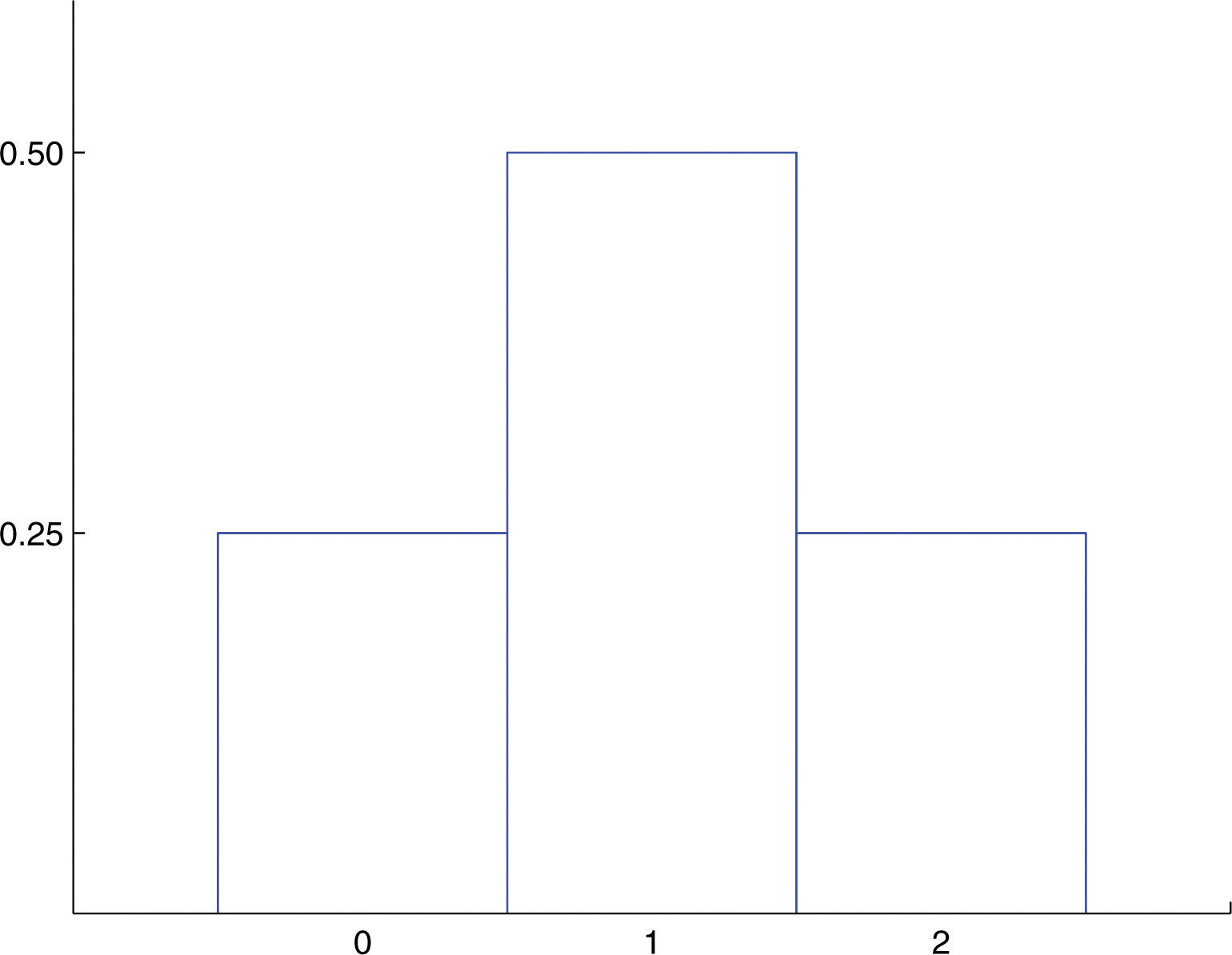
A fair coin is tossed twice. Let X be the number of heads that are observed.
- Construct the probability distribution of X.
- Find the probability that at least one head is observed.
Solution:
-
The possible values that X can take are 0, 1, and 2. Each of these numbers corresponds to an event in the sample space of equally likely outcomes for this experiment: X = 0 to , X = 1 to , and X = 2 to The probability of each of these events, hence of the corresponding value of X, can be found simply by counting, to give
This table is the probability distribution of X.
-
“At least one head” is the event X ≥ 1, which is the union of the mutually exclusive events X = 1 and X = 2. Thus
A histogram that graphically illustrates the probability distribution is given in Figure 4.1 "Probability Distribution for Tossing a Fair Coin Twice".
Figure 4.1 Probability Distribution for Tossing a Fair Coin Twice
Example 2
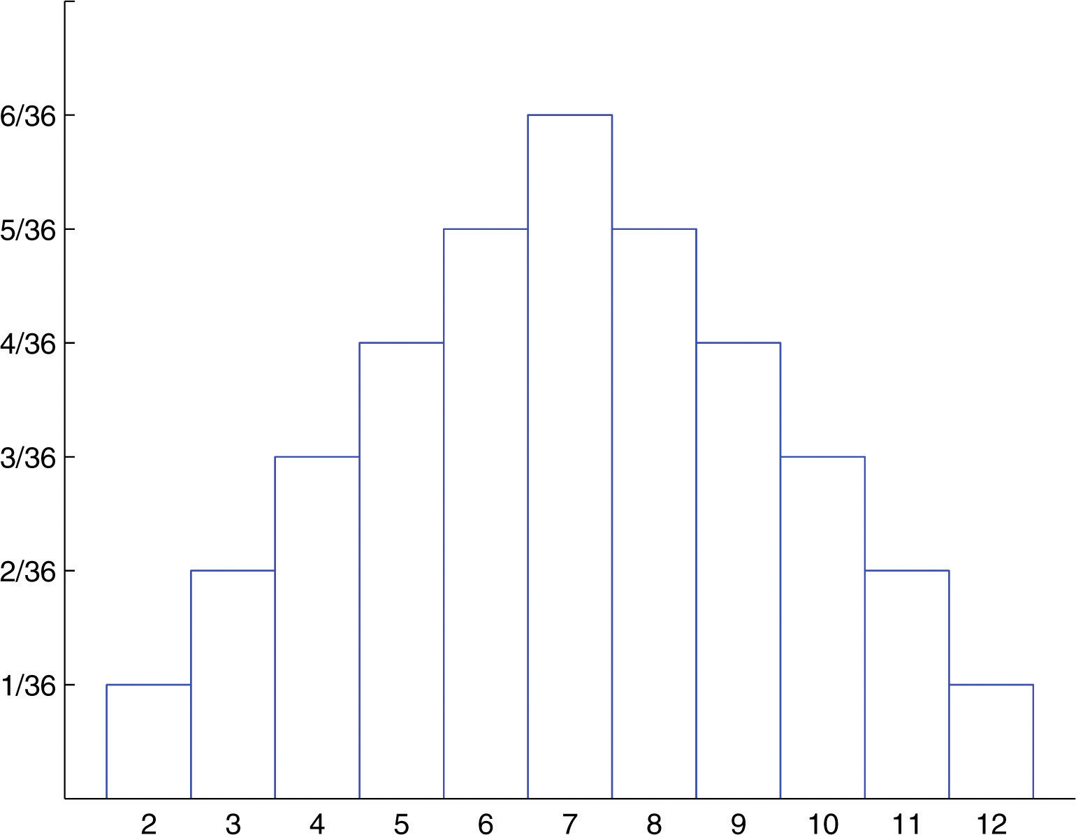
A pair of fair dice is rolled. Let X denote the sum of the number of dots on the top faces.
- Construct the probability distribution of X.
- Find P(X ≥ 9).
- Find the probability that X takes an even value.
Solution:
The sample space of equally likely outcomes is
-
The possible values for X are the numbers 2 through 12. X = 2 is the event {11}, so X = 3 is the event {12,21}, so Continuing this way we obtain the table
This table is the probability distribution of X.
-
The event X ≥ 9 is the union of the mutually exclusive events X = 9, X = 10, X = 11, and X = 12. Thus
-
Before we immediately jump to the conclusion that the probability that X takes an even value must be 0.5, note that X takes six different even values but only five different odd values. We compute
A histogram that graphically illustrates the probability distribution is given in Figure 4.2 "Probability Distribution for Tossing Two Fair Dice".
Figure 4.2 Probability Distribution for Tossing Two Fair Dice
The Mean and Standard Deviation of a Discrete Random Variable
Definition
The meanThe number , measuring its average upon repeated trials. (also called the expected valueIts mean.) of a discrete random variable X is the number
The mean of a random variable may be interpreted as the average of the values assumed by the random variable in repeated trials of the experiment.
Example 3
Find the mean of the discrete random variable X whose probability distribution is
Solution:
The formula in the definition gives
Example 4
A service organization in a large town organizes a raffle each month. One thousand raffle tickets are sold for $1 each. Each has an equal chance of winning. First prize is $300, second prize is $200, and third prize is $100. Let X denote the net gain from the purchase of one ticket.
- Construct the probability distribution of X.
- Find the probability of winning any money in the purchase of one ticket.
- Find the expected value of X, and interpret its meaning.
Solution:
-
If a ticket is selected as the first prize winner, the net gain to the purchaser is the $300 prize less the $1 that was paid for the ticket, hence X = 300 − 1 = 299. There is one such ticket, so P(299) = 0.001. Applying the same “income minus outgo” principle to the second and third prize winners and to the 997 losing tickets yields the probability distribution:
-
Let W denote the event that a ticket is selected to win one of the prizes. Using the table
-
Using the formula in the definition of expected value,
The negative value means that one loses money on the average. In particular, if someone were to buy tickets repeatedly, then although he would win now and then, on average he would lose 40 cents per ticket purchased.
The concept of expected value is also basic to the insurance industry, as the following simplified example illustrates.
Example 5
A life insurance company will sell a $200,000 one-year term life insurance policy to an individual in a particular risk group for a premium of $195. Find the expected value to the company of a single policy if a person in this risk group has a 99.97% chance of surviving one year.
Solution:
Let X denote the net gain to the company from the sale of one such policy. There are two possibilities: the insured person lives the whole year or the insured person dies before the year is up. Applying the “income minus outgo” principle, in the former case the value of X is 195 − 0; in the latter case it is Since the probability in the first case is 0.9997 and in the second case is , the probability distribution for X is:
Therefore
Occasionally (in fact, 3 times in 10,000) the company loses a large amount of money on a policy, but typically it gains $195, which by our computation of works out to a net gain of $135 per policy sold, on average.
Definition
The variance, , of a discrete random variable X is the number
which by algebra is equivalent to the formula
Definition
The standard deviationThe number (also computed using ), measuring its variability under repeated trials., σ, of a discrete random variable X is the square root of its variance, hence is given by the formulas
The variance and standard deviation of a discrete random variable X may be interpreted as measures of the variability of the values assumed by the random variable in repeated trials of the experiment. The units on the standard deviation match those of X.
Example 6
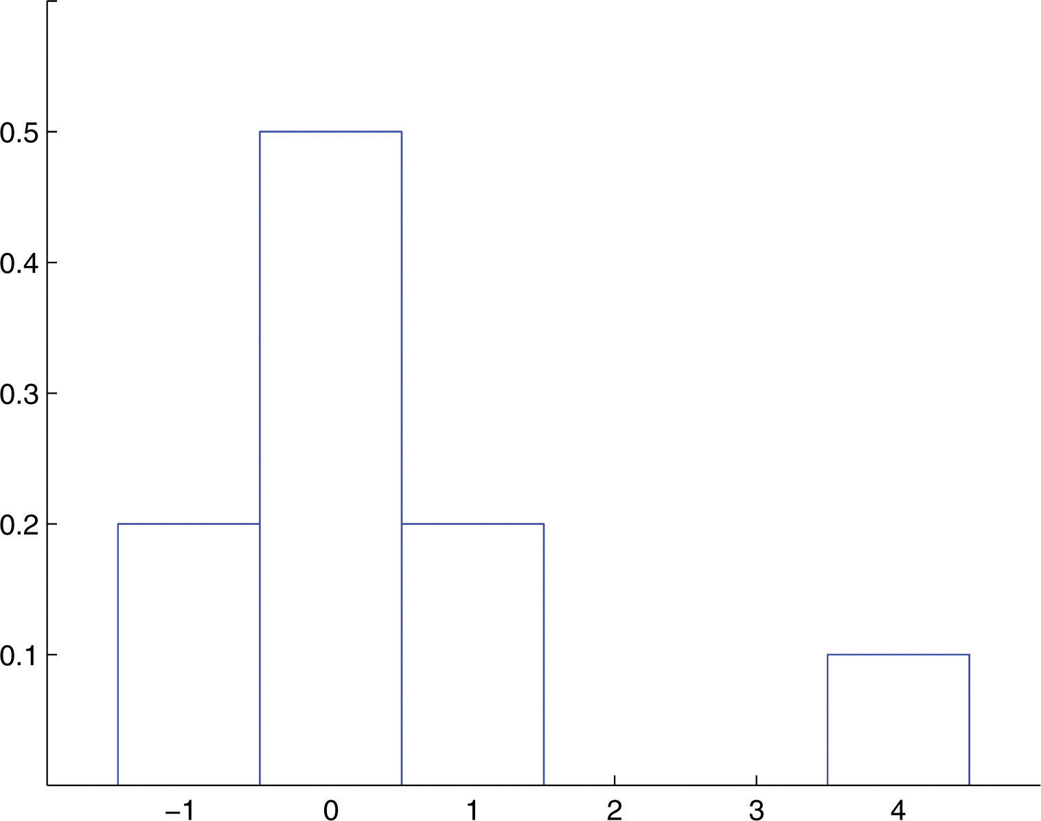
A discrete random variable X has the following probability distribution:
A histogram that graphically illustrates the probability distribution is given in Figure 4.3 "Probability Distribution of a Discrete Random Variable".
Figure 4.3 Probability Distribution of a Discrete Random Variable
Compute each of the following quantities.
- a.
- P(X > 0).
- P(X ≥ 0).
- The mean μ of X.
- The variance of X.
- The standard deviation σ of X.
Solution:
- Since all probabilities must add up to 1,
- Directly from the table,
- From the table,
- From the table,
- Since none of the numbers listed as possible values for X is less than or equal to −2, the event X ≤ −2 is impossible, so P(X ≤ −2) = 0.
-
Using the formula in the definition of μ,
-
Using the formula in the definition of and the value of μ that was just computed,
- Using the result of part (g),
Key Takeaways
- The probability distribution of a discrete random variable X is a listing of each possible value x taken by X along with the probability that X takes that value in one trial of the experiment.
- The mean μ of a discrete random variable X is a number that indicates the average value of X over numerous trials of the experiment. It is computed using the formula
- The variance and standard deviation σ of a discrete random variable X are numbers that indicate the variability of X over numerous trials of the experiment. They may be computed using the formula , taking the square root to obtain σ.
Exercises
-
Determine whether or not the table is a valid probability distribution of a discrete random variable. Explain fully.
-
-
Determine whether or not the table is a valid probability distribution of a discrete random variable. Explain fully.
-
-
A discrete random variable X has the following probability distribution:
Compute each of the following quantities.
- P(X > 80).
- P(X ≤ 80).
- The mean μ of X.
- The variance of X.
- The standard deviation σ of X.
-
A discrete random variable X has the following probability distribution:
Compute each of the following quantities.
- P(X > 18).
- P(X ≤ 18).
- The mean μ of X.
- The variance of X.
- The standard deviation σ of X.
-
If each die in a pair is “loaded” so that one comes up half as often as it should, six comes up half again as often as it should, and the probabilities of the other faces are unaltered, then the probability distribution for the sum X of the number of dots on the top faces when the two are rolled is
Compute each of the following.
- P(X ≥ 7).
- The mean μ of X. (For fair dice this number is 7.)
- The standard deviation σ of X. (For fair dice this number is about 2.415.)
Basic
-
Borachio works in an automotive tire factory. The number X of sound but blemished tires that he produces on a random day has the probability distribution
- Find the probability that Borachio will produce more than three blemished tires tomorrow.
- Find the probability that Borachio will produce at most two blemished tires tomorrow.
- Compute the mean and standard deviation of X. Interpret the mean in the context of the problem.
-
In a hamster breeder's experience the number X of live pups in a litter of a female not over twelve months in age who has not borne a litter in the past six weeks has the probability distribution
- Find the probability that the next litter will produce five to seven live pups.
- Find the probability that the next litter will produce at least six live pups.
- Compute the mean and standard deviation of X. Interpret the mean in the context of the problem.
-
The number X of days in the summer months that a construction crew cannot work because of the weather has the probability distribution
- Find the probability that no more than ten days will be lost next summer.
- Find the probability that from 8 to 12 days will be lost next summer.
- Find the probability that no days at all will be lost next summer.
- Compute the mean and standard deviation of X. Interpret the mean in the context of the problem.
-
Let X denote the number of boys in a randomly selected three-child family. Assuming that boys and girls are equally likely, construct the probability distribution of X.
-
Let X denote the number of times a fair coin lands heads in three tosses. Construct the probability distribution of X.
-
Five thousand lottery tickets are sold for $1 each. One ticket will win $1,000, two tickets will win $500 each, and ten tickets will win $100 each. Let X denote the net gain from the purchase of a randomly selected ticket.
- Construct the probability distribution of X.
- Compute the expected value of X. Interpret its meaning.
- Compute the standard deviation σ of X.
-
Seven thousand lottery tickets are sold for $5 each. One ticket will win $2,000, two tickets will win $750 each, and five tickets will win $100 each. Let X denote the net gain from the purchase of a randomly selected ticket.
- Construct the probability distribution of X.
- Compute the expected value of X. Interpret its meaning.
- Compute the standard deviation σ of X.
-
An insurance company will sell a $90,000 one-year term life insurance policy to an individual in a particular risk group for a premium of $478. Find the expected value to the company of a single policy if a person in this risk group has a 99.62% chance of surviving one year.
-
An insurance company will sell a $10,000 one-year term life insurance policy to an individual in a particular risk group for a premium of $368. Find the expected value to the company of a single policy if a person in this risk group has a 97.25% chance of surviving one year.
-
An insurance company estimates that the probability that an individual in a particular risk group will survive one year is 0.9825. Such a person wishes to buy a $150,000 one-year term life insurance policy. Let C denote how much the insurance company charges such a person for such a policy.
- Construct the probability distribution of X. (Two entries in the table will contain C.)
- Compute the expected value of X.
- Determine the value C must have in order for the company to break even on all such policies (that is, to average a net gain of zero per policy on such policies).
- Determine the value C must have in order for the company to average a net gain of $250 per policy on all such policies.
-
An insurance company estimates that the probability that an individual in a particular risk group will survive one year is 0.99. Such a person wishes to buy a $75,000 one-year term life insurance policy. Let C denote how much the insurance company charges such a person for such a policy.
- Construct the probability distribution of X. (Two entries in the table will contain C.)
- Compute the expected value of X.
- Determine the value C must have in order for the company to break even on all such policies (that is, to average a net gain of zero per policy on such policies).
- Determine the value C must have in order for the company to average a net gain of $150 per policy on all such policies.
-
A roulette wheel has 38 slots. Thirty-six slots are numbered from 1 to 36; half of them are red and half are black. The remaining two slots are numbered 0 and 00 and are green. In a $1 bet on red, the bettor pays $1 to play. If the ball lands in a red slot, he receives back the dollar he bet plus an additional dollar. If the ball does not land on red he loses his dollar. Let X denote the net gain to the bettor on one play of the game.
- Construct the probability distribution of X.
- Compute the expected value of X, and interpret its meaning in the context of the problem.
- Compute the standard deviation of X.
-
A roulette wheel has 38 slots. Thirty-six slots are numbered from 1 to 36; the remaining two slots are numbered 0 and 00. Suppose the “number” 00 is considered not to be even, but the number 0 is still even. In a $1 bet on even, the bettor pays $1 to play. If the ball lands in an even numbered slot, he receives back the dollar he bet plus an additional dollar. If the ball does not land on an even numbered slot, he loses his dollar. Let X denote the net gain to the bettor on one play of the game.
- Construct the probability distribution of X.
- Compute the expected value of X, and explain why this game is not offered in a casino (where 0 is not considered even).
- Compute the standard deviation of X.
-
The time, to the nearest whole minute, that a city bus takes to go from one end of its route to the other has the probability distribution shown. As sometimes happens with probabilities computed as empirical relative frequencies, probabilities in the table add up only to a value other than 1.00 because of round-off error.
- Find the average time the bus takes to drive the length of its route.
- Find the standard deviation of the length of time the bus takes to drive the length of its route.
-
Tybalt receives in the mail an offer to enter a national sweepstakes. The prizes and chances of winning are listed in the offer as: $5 million, one chance in 65 million; $150,000, one chance in 6.5 million; $5,000, one chance in 650,000; and $1,000, one chance in 65,000. If it costs Tybalt 44 cents to mail his entry, what is the expected value of the sweepstakes to him?
Applications
-
The number X of nails in a randomly selected 1-pound box has the probability distribution shown. Find the average number of nails per pound.
-
Three fair dice are rolled at once. Let X denote the number of dice that land with the same number of dots on top as at least one other die. The probability distribution for X is
- Find the missing value u of X.
- Find the missing probability p.
- Compute the mean of X.
- Compute the standard deviation of X.
-
Two fair dice are rolled at once. Let X denote the difference in the number of dots that appear on the top faces of the two dice. Thus for example if a one and a five are rolled, X = 4, and if two sixes are rolled, X = 0.
- Construct the probability distribution for X.
- Compute the mean μ of X.
- Compute the standard deviation σ of X.
-
A fair coin is tossed repeatedly until either it lands heads or a total of five tosses have been made, whichever comes first. Let X denote the number of tosses made.
- Construct the probability distribution for X.
- Compute the mean μ of X.
- Compute the standard deviation σ of X.
-
A manufacturer receives a certain component from a supplier in shipments of 100 units. Two units in each shipment are selected at random and tested. If either one of the units is defective the shipment is rejected. Suppose a shipment has 5 defective units.
- Construct the probability distribution for the number X of defective units in such a sample. (A tree diagram is helpful.)
- Find the probability that such a shipment will be accepted.
-
Shylock enters a local branch bank at 4:30 p.m. every payday, at which time there are always two tellers on duty. The number X of customers in the bank who are either at a teller window or are waiting in a single line for the next available teller has the following probability distribution.
- What number of customers does Shylock most often see in the bank the moment he enters?
- What number of customers waiting in line does Shylock most often see the moment he enters?
- What is the average number of customers who are waiting in line the moment Shylock enters?
-
The owner of a proposed outdoor theater must decide whether to include a cover that will allow shows to be performed in all weather conditions. Based on projected audience sizes and weather conditions, the probability distribution for the revenue X per night if the cover is not installed is
The additional cost of the cover is $410,000. The owner will have it built if this cost can be recovered from the increased revenue the cover affords in the first ten 90-night seasons.
- Compute the mean revenue per night if the cover is not installed.
- Use the answer to (a) to compute the projected total revenue per 90-night season if the cover is not installed.
- Compute the projected total revenue per season when the cover is in place. To do so assume that if the cover were in place the revenue each night of the season would be the same as the revenue on a clear night.
- Using the answers to (b) and (c), decide whether or not the additional cost of the installation of the cover will be recovered from the increased revenue over the first ten years. Will the owner have the cover installed?
Additional Exercises
Answers
-
- no: the sum of the probabilities exceeds 1
- no: a negative probability
- no: the sum of the probabilities is less than 1
-
-
- 0.4
- 0.1
- 0.9
- 79.15
- σ = 1.2359
-
-
- 0.6528
- 0.7153
- μ = 7.8333
- σ = 2.3424
-
-
- 0.79
- 0.60
- μ = 5.8, σ = 1.2570
-
-
-
-
-
- −0.4
- 17.8785
-
-
-
136
-
-
-
- C ≥ 2625
- C ≥ 2875
-
-
-
-
- In many bets the bettor sustains an average loss of about 5.25 cents per bet.
- 0.9986
-
-
-
- 43.54
- 1.2046
-
-
101.02
-
-
-
- 1.9444
- 1.4326
-
-
-
-
- 0.902
-
-
-
- 2523.25
- 227,092.5
- 270,000
- The owner will install the cover.
4.3 The Binomial Distribution
Learning Objectives
- To learn the concept of a binomial random variable.
- To learn how to recognize a random variable as being a binomial random variable.
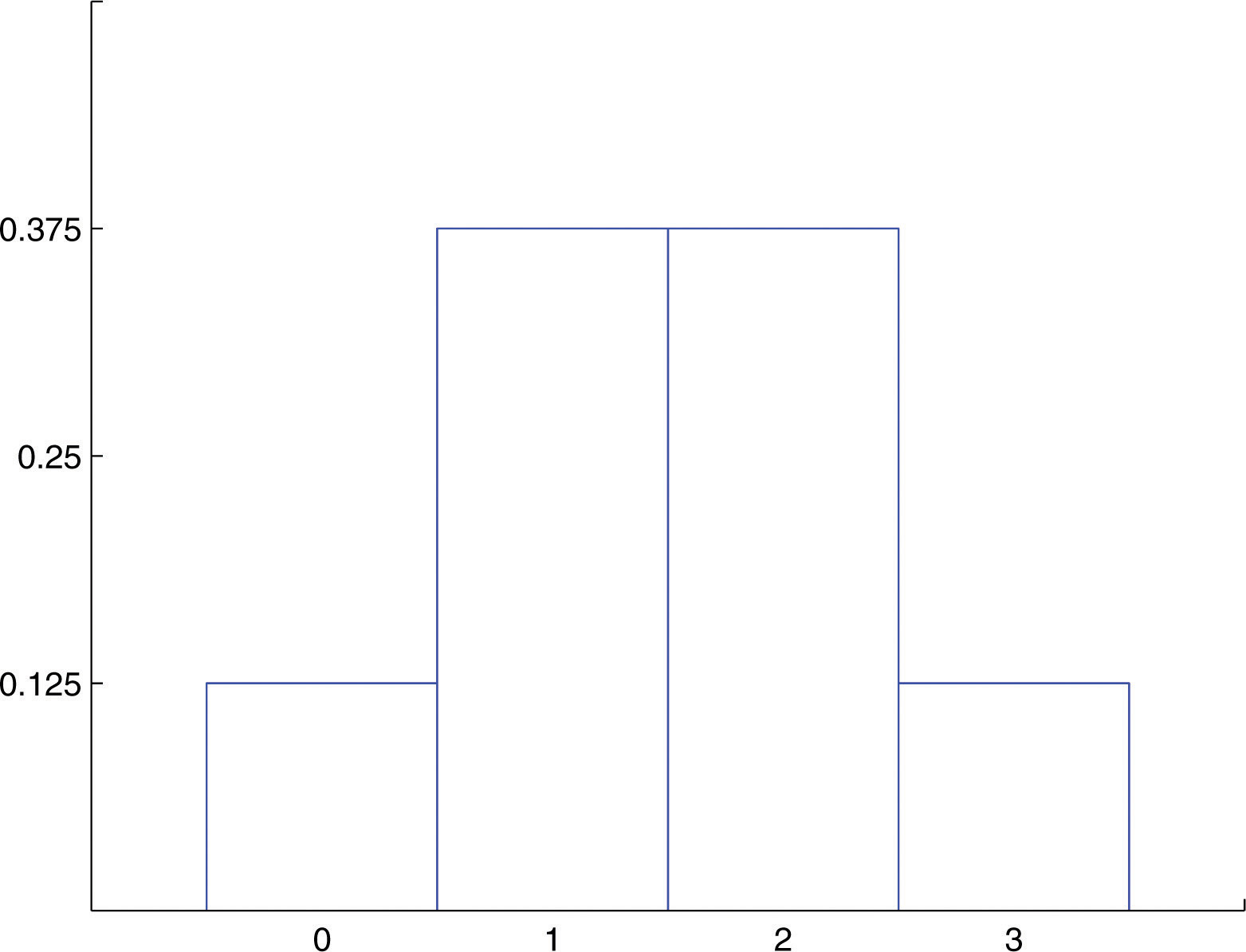
The experiment of tossing a fair coin three times and the experiment of observing the genders according to birth order of the children in a randomly selected three-child family are completely different, but the random variables that count the number of heads in the coin toss and the number of boys in the family (assuming the two genders are equally likely) are the same random variable, the one with probability distribution
A histogram that graphically illustrates this probability distribution is given in Figure 4.4 "Probability Distribution for Three Coins and Three Children". What is common to the two experiments is that we perform three identical and independent trials of the same action, each trial has only two outcomes (heads or tails, boy or girl), and the probability of success is the same number, 0.5, on every trial. The random variable that is generated is called the binomial random variableA random variable that counts successes in a fixed number of independent, identical trials of a success/failure experiment. with parameters n = 3 and p = 0.5. This is just one case of a general situation.
Figure 4.4 Probability Distribution for Three Coins and Three Children
Definition
Suppose a random experiment has the following characteristics.
- There are n identical and independent trials of a common procedure.
- There are exactly two possible outcomes for each trial, one termed “success” and the other “failure.”
- The probability of success on any one trial is the same number p.
Then the discrete random variable X that counts the number of successes in the n trials is the binomial random variable with parameters n and p. We also say that X has a binomial distribution with parameters n and p.
The following four examples illustrate the definition. Note how in every case “success” is the outcome that is counted, not the outcome that we prefer or think is better in some sense.
- A random sample of 125 students is selected from a large college in which the proportion of students who are females is 57%. Suppose X denotes the number of female students in the sample. In this situation there are n = 125 identical and independent trials of a common procedure, selecting a student at random; there are exactly two possible outcomes for each trial, “success” (what we are counting, that the student be female) and “failure;” and finally the probability of success on any one trial is the same number p = 0.57. X is a binomial random variable with parameters n = 125 and p = 0.57.
- A multiple-choice test has 15 questions, each of which has five choices. An unprepared student taking the test answers each of the questions completely randomly by choosing an arbitrary answer from the five provided. Suppose X denotes the number of answers that the student gets right. X is a binomial random variable with parameters n = 15 and
- In a survey of 1,000 registered voters each voter is asked if he intends to vote for a candidate Titania Queen in the upcoming election. Suppose X denotes the number of voters in the survey who intend to vote for Titania Queen. X is a binomial random variable with n = 1000 and p equal to the true proportion of voters (surveyed or not) who intend to vote for Titania Queen.
- An experimental medication was given to 30 patients with a certain medical condition. Suppose X denotes the number of patients who develop severe side effects. X is a binomial random variable with n = 30 and p equal to the true probability that a patient with the underlying condition will experience severe side effects if given that medication.
Probability Formula for a Binomial Random Variable
Often the most difficult aspect of working a problem that involves the binomial random variable is recognizing that the random variable in question has a binomial distribution. Once that is known, probabilities can be computed using the following formula.
If X is a binomial random variable with parameters n and p, then
where and where for any counting number m, (read “m factorial”) is defined by
and in general
Example 7
Seventeen percent of victims of financial fraud know the perpetrator of the fraud personally.
- Use the formula to construct the probability distribution for the number X of people in a random sample of five victims of financial fraud who knew the perpetrator personally.
- A investigator examines five cases of financial fraud every day. Find the most frequent number of cases each day in which the victim knew the perpetrator.
- A investigator examines five cases of financial fraud every day. Find the average number of cases per day in which the victim knew the perpetrator.
Solution:
-
The random variable X is binomial with parameters n = 5 and p = 0.17; The possible values of X are 0, 1, 2, 3, 4, and 5.
The remaining three probabilities are computed similarly, to give the probability distribution
The probabilities do not add up to exactly 1 because of rounding.
This probability distribution is represented by the histogram in Figure 4.5 "Probability Distribution of the Binomial Random Variable in ", which graphically illustrates just how improbable the events X = 4 and X = 5 are. The corresponding bar in the histogram above the number 4 is barely visible, if visible at all, and the bar above 5 is far too short to be visible.
Figure 4.5 Probability Distribution of the Binomial Random Variable in Note 4.29 "Example 7"
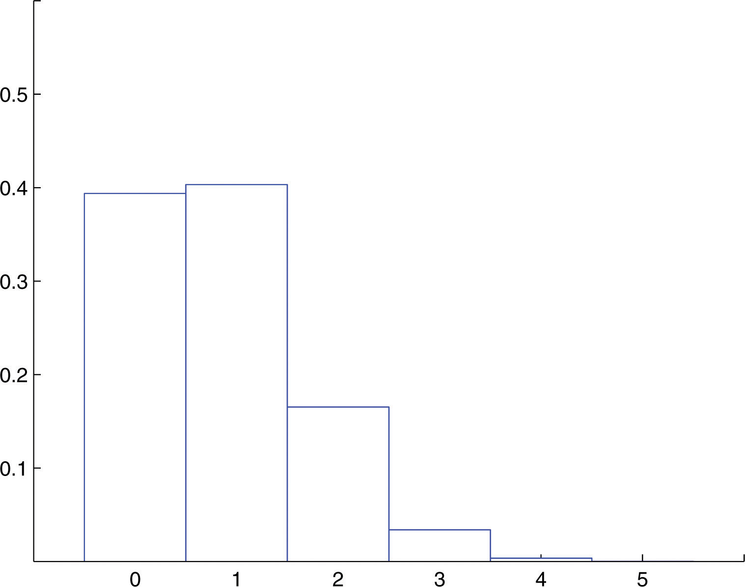
- The value of X that is most likely is X = 1, so the most frequent number of cases seen each day in which the victim knew the perpetrator is one.
-
The average number of cases per day in which the victim knew the perpetrator is the mean of X, which is
Special Formulas for the Mean and Standard Deviation of a Binomial Random Variable
Since a binomial random variable is a discrete random variable, the formulas for its mean, variance, and standard deviation given in the previous section apply to it, as we just saw in Note 4.29 "Example 7" in the case of the mean. However, for the binomial random variable there are much simpler formulas.
If X is a binomial random variable with parameters n and p, then
where
Example 8
Find the mean and standard deviation of the random variable X of Note 4.29 "Example 7".
Solution:
The random variable X is binomial with parameters n = 5 and p = 0.17, and Thus its mean and standard deviation are
and
The Cumulative Probability Distribution of a Binomial Random Variable
In order to allow a broader range of more realistic problems Chapter 12 "Appendix" contains probability tables for binomial random variables for various choices of the parameters n and p. These tables are not the probability distributions that we have seen so far, but are cumulative probability distributions. In the place of the probability the table contains the probability
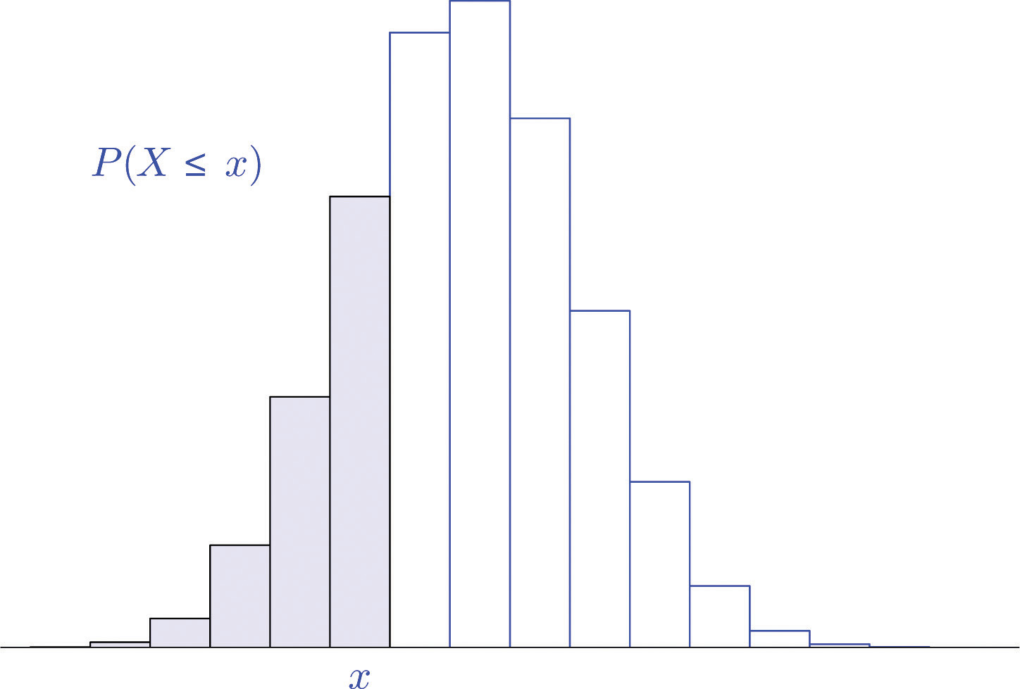
This is illustrated in Figure 4.6 "Cumulative Probabilities". The probability entered in the table corresponds to the area of the shaded region. The reason for providing a cumulative table is that in practical problems that involve a binomial random variable typically the probability that is sought is of the form or The cumulative table is much easier to use for computing since all the individual probabilities have already been computed and added. The one table suffices for both or and can be used to readily obtain probabilities of the form , too, because of the following formulas. The first is just the Probability Rule for Complements.
Figure 4.6 Cumulative Probabilities
If X is a discrete random variable, then
Example 9
A student takes a ten-question true/false exam.
- Find the probability that the student gets exactly six of the questions right simply by guessing the answer on every question.
- Find the probability that the student will obtain a passing grade of 60% or greater simply by guessing.
Solution:
Let X denote the number of questions that the student guesses correctly. Then X is a binomial random variable with parameters n = 10 and p = 0.50.
-
The probability sought is The formula gives
Using the table,
-
The student must guess correctly on at least 60% of the questions, which is questions. The probability sought is not (an easy mistake to make), but
Instead of computing each of these five numbers using the formula and adding them we can use the table to obtain
which is much less work and of sufficient accuracy for the situation at hand.
Example 10
An appliance repairman services five washing machines on site each day. One-third of the service calls require installation of a particular part.
- The repairman has only one such part on his truck today. Find the probability that the one part will be enough today, that is, that at most one washing machine he services will require installation of this particular part.
- Find the minimum number of such parts he should take with him each day in order that the probability that he have enough for the day's service calls is at least 95%.
Solution:
Let X denote the number of service calls today on which the part is required. Then X is a binomial random variable with parameters n = 5 and
-
Note that the probability in question is not , but rather P(X ≤ 1). Using the cumulative distribution table in Chapter 12 "Appendix",
- The answer is the smallest number x such that the table entry is at least 0.9500. Since is less than 0.95, two parts are not enough. Since is as large as 0.95, three parts will suffice at least 95% of the time. Thus the minimum needed is three.
Key Takeaways
- The discrete random variable X that counts the number of successes in n identical, independent trials of a procedure that always results in either of two outcomes, “success” or “failure,” and in which the probability of success on each trial is the same number p, is called the binomial random variable with parameters n and p.
- There is a formula for the probability that the binomial random variable with parameters n and p will take a particular value x.
- There are special formulas for the mean, variance, and standard deviation of the binomial random variable with parameters n and p that are much simpler than the general formulas that apply to all discrete random variables.
- Cumulative probability distribution tables, when available, facilitate computation of probabilities encountered in typical practical situations.
Exercises
-
Determine whether or not the random variable X is a binomial random variable. If so, give the values of n and p. If not, explain why not.
- X is the number of dots on the top face of fair die that is rolled.
- X is the number of hearts in a five-card hand drawn (without replacement) from a well-shuffled ordinary deck.
- X is the number of defective parts in a sample of ten randomly selected parts coming from a manufacturing process in which 0.02% of all parts are defective.
- X is the number of times the number of dots on the top face of a fair die is even in six rolls of the die.
- X is the number of dice that show an even number of dots on the top face when six dice are rolled at once.
-
Determine whether or not the random variable X is a binomial random variable. If so, give the values of n and p. If not, explain why not.
- X is the number of black marbles in a sample of 5 marbles drawn randomly and without replacement from a box that contains 25 white marbles and 15 black marbles.
- X is the number of black marbles in a sample of 5 marbles drawn randomly and with replacement from a box that contains 25 white marbles and 15 black marbles.
- X is the number of voters in favor of proposed law in a sample 1,200 randomly selected voters drawn from the entire electorate of a country in which 35% of the voters favor the law.
- X is the number of fish of a particular species, among the next ten landed by a commercial fishing boat, that are more than 13 inches in length, when 17% of all such fish exceed 13 inches in length.
- X is the number of coins that match at least one other coin when four coins are tossed at once.
-
X is a binomial random variable with parameters n = 12 and p = 0.82. Compute the probability indicated.
-
X is a binomial random variable with parameters n = 16 and p = 0.74. Compute the probability indicated.
-
X is a binomial random variable with parameters n = 5, p = 0.5. Use the tables in Chapter 12 "Appendix" to compute the probability indicated.
- P(X ≤ 3)
- P(X ≥ 3)
-
X is a binomial random variable with parameters n = 5, Use the table in Chapter 12 "Appendix" to compute the probability indicated.
- P(X ≤ 2)
- P(X ≥ 2)
-
X is a binomial random variable with the parameters shown. Use the tables in Chapter 12 "Appendix" to compute the probability indicated.
- n = 10, p = 0.25, P(X ≤ 6)
- n = 10, p = 0.75, P(X ≤ 6)
- n = 15, p = 0.75, P(X ≤ 6)
- n = 15, p = 0.75,
- n = 15, ,
-
X is a binomial random variable with the parameters shown. Use the tables in Chapter 12 "Appendix" to compute the probability indicated.
- n = 5, p = 0.05, P(X ≤ 1)
- n = 5, p = 0.5, P(X ≤ 1)
- n = 10, p = 0.75, P(X ≤ 5)
- n = 10, p = 0.75,
- n = 10, ,
-
X is a binomial random variable with the parameters shown. Use the special formulas to compute its mean μ and standard deviation σ.
- n = 8, p = 0.43
- n = 47, p = 0.82
- n = 1200, p = 0.44
- n = 2100, p = 0.62
-
X is a binomial random variable with the parameters shown. Use the special formulas to compute its mean μ and standard deviation σ.
- n = 14, p = 0.55
- n = 83, p = 0.05
- n = 957, p = 0.35
- n = 1750, p = 0.79
-
X is a binomial random variable with the parameters shown. Compute its mean μ and standard deviation σ in two ways, first using the tables in Chapter 12 "Appendix" in conjunction with the general formulas and , then using the special formulas and
- n = 5,
- n = 10, p = 0.75
-
X is a binomial random variable with the parameters shown. Compute its mean μ and standard deviation σ in two ways, first using the tables in Chapter 12 "Appendix" in conjunction with the general formulas and , then using the special formulas and
- n = 10, p = 0.25
- n = 15, p = 0.1
-
X is a binomial random variable with parameters n = 10 and Use the cumulative probability distribution for X that is given in Chapter 12 "Appendix" to construct the probability distribution of X.
-
X is a binomial random variable with parameters n = 15 and Use the cumulative probability distribution for X that is given in Chapter 12 "Appendix" to construct the probability distribution of X.
-
In a certain board game a player's turn begins with three rolls of a pair of dice. If the player rolls doubles all three times there is a penalty. The probability of rolling doubles in a single roll of a pair of fair dice is 1/6. Find the probability of rolling doubles all three times.
-
A coin is bent so that the probability that it lands heads up is 2/3. The coin is tossed ten times.
- Find the probability that it lands heads up at most five times.
- Find the probability that it lands heads up more times than it lands tails up.
Basic
-
An English-speaking tourist visits a country in which 30% of the population speaks English. He needs to ask someone directions.
- Find the probability that the first person he encounters will be able to speak English.
- The tourist sees four local people standing at a bus stop. Find the probability that at least one of them will be able to speak English.
-
The probability that an egg in a retail package is cracked or broken is 0.025.
- Find the probability that a carton of one dozen eggs contains no eggs that are either cracked or broken.
- Find the probability that a carton of one dozen eggs has (i) at least one that is either cracked or broken; (ii) at least two that are cracked or broken.
- Find the average number of cracked or broken eggs in one dozen cartons.
-
An appliance store sells 20 refrigerators each week. Ten percent of all purchasers of a refrigerator buy an extended warranty. Let X denote the number of the next 20 purchasers who do so.
- Verify that X satisfies the conditions for a binomial random variable, and find n and p.
- Find the probability that X is zero.
- Find the probability that X is two, three, or four.
- Find the probability that X is at least five.
-
Adverse growing conditions have caused 5% of grapefruit grown in a certain region to be of inferior quality. Grapefruit are sold by the dozen.
- Find the average number of inferior quality grapefruit per box of a dozen.
- A box that contains two or more grapefruit of inferior quality will cause a strong adverse customer reaction. Find the probability that a box of one dozen grapefruit will contain two or more grapefruit of inferior quality.
-
The probability that a 7-ounce skein of a discount worsted weight knitting yarn contains a knot is 0.25. Goneril buys ten skeins to crochet an afghan.
- Find the probability that (i) none of the ten skeins will contain a knot; (ii) at most one will.
- Find the expected number of skeins that contain knots.
- Find the most likely number of skeins that contain knots.
-
One-third of all patients who undergo a non-invasive but unpleasant medical test require a sedative. A laboratory performs 20 such tests daily. Let X denote the number of patients on any given day who require a sedative.
- Verify that X satisfies the conditions for a binomial random variable, and find n and p.
- Find the probability that on any given day between five and nine patients will require a sedative (include five and nine).
- Find the average number of patients each day who require a sedative.
- Using the cumulative probability distribution for X in Chapter 12 "Appendix", find the minimum number of doses of the sedative that should be on hand at the start of the day so that there is a 99% chance that the laboratory will not run out.
-
About 2% of alumni give money upon receiving a solicitation from the college or university from which they graduated. Find the average number monetary gifts a college can expect from every 2,000 solicitations it sends.
-
Of all college students who are eligible to give blood, about 18% do so on a regular basis. Each month a local blood bank sends an appeal to give blood to 250 randomly selected students. Find the average number of appeals in such mailings that are made to students who already give blood.
-
About 12% of all individuals write with their left hands. A class of 130 students meets in a classroom with 130 individual desks, exactly 14 of which are constructed for people who write with their left hands. Find the probability that exactly 14 of the students enrolled in the class write with their left hands.
-
A travelling salesman makes a sale on 65% of his calls on regular customers. He makes four sales calls each day.
- Construct the probability distribution of X, the number of sales made each day.
- Find the probability that, on a randomly selected day, the salesman will make a sale.
- Assuming that the salesman makes 20 sales calls per week, find the mean and standard deviation of the number of sales made per week.
-
A corporation has advertised heavily to try to insure that over half the adult population recognizes the brand name of its products. In a random sample of 20 adults, 14 recognized its brand name. What is the probability that 14 or more people in such a sample would recognize its brand name if the actual proportion p of all adults who recognize the brand name were only 0.50?
Applications
-
When dropped on a hard surface a thumbtack lands with its sharp point touching the surface with probability 2/3; it lands with its sharp point directed up into the air with probability 1/3. The tack is dropped and its landing position observed 15 times.
- Find the probability that it lands with its point in the air at least 7 times.
- If the experiment of dropping the tack 15 times is done repeatedly, what is the average number of times it lands with its point in the air?
-
A professional proofreader has a 98% chance of detecting an error in a piece of written work (other than misspellings, double words, and similar errors that are machine detected). A work contains four errors.
- Find the probability that the proofreader will miss at least one of them.
- Show that two such proofreaders working independently have a 99.96% chance of detecting an error in a piece of written work.
- Find the probability that two such proofreaders working independently will miss at least one error in a work that contains four errors.
-
A multiple choice exam has 20 questions; there are four choices for each question.
- A student guesses the answer to every question. Find the chance that he guesses correctly between four and seven times.
- Find the minimum score the instructor can set so that the probability that a student will pass just by guessing is 20% or less.
-
In spite of the requirement that all dogs boarded in a kennel be inoculated, the chance that a healthy dog boarded in a clean, well-ventilated kennel will develop kennel cough from a carrier is 0.008.
- If a carrier (not known to be such, of course) is boarded with three other dogs, what is the probability that at least one of the three healthy dogs will develop kennel cough?
- If a carrier is boarded with four other dogs, what is the probability that at least one of the four healthy dogs will develop kennel cough?
- The pattern evident from parts (a) and (b) is that if dogs are boarded together, one a carrier and K healthy dogs, then the probability that at least one of the healthy dogs will develop kennel cough is , where X is the binomial random variable that counts the number of healthy dogs that develop the condition. Experiment with different values of K in this formula to find the maximum number of dogs that a kennel owner can board together so that if one of the dogs has the condition, the chance that another dog will be infected is less than 0.05.
-
Investigators need to determine which of 600 adults have a medical condition that affects 2% of the adult population. A blood sample is taken from each of the individuals.
- Show that the expected number of diseased individuals in the group of 600 is 12 individuals.
- Instead of testing all 600 blood samples to find the expected 12 diseased individuals, investigators group the samples into 60 groups of 10 each, mix a little of the blood from each of the 10 samples in each group, and test each of the 60 mixtures. Show that the probability that any such mixture will contain the blood of at least one diseased person, hence test positive, is about 0.18.
- Based on the result in (b), show that the expected number of mixtures that test positive is about 11. (Supposing that indeed 11 of the 60 mixtures test positive, then we know that none of the 490 persons whose blood was in the remaining 49 samples that tested negative has the disease. We have eliminated 490 persons from our search while performing only 60 tests.)
Additional Exercises
Answers
-
- not binomial; not success/failure.
- not binomial; trials are not independent.
- binomial; n = 10, p = 0.0002
- binomial; n = 6, p = 0.5
- binomial; n = 6, p = 0.5
-
-
- 0.2434
- 0.2151
- 0
-
-
- 0.8125
- 0.5000
- 0.3125
- 0.0313
- 0.0312
-
-
- 0.9965
- 0.2241
- 0.0042
- 0.2252
- 0.5390
-
-
- μ = 3.44, σ = 1.4003
- μ = 38.54, σ = 2.6339
- μ = 528, σ = 17.1953
- μ = 1302, σ = 22.2432
-
-
- μ = 1.6667, σ = 1.0541
- μ = 7.5, σ = 1.3693
-
-
-
-
0.0046
-
-
- 0.3
- 0.7599
-
-
- n = 20, p = 0.1
- 0.1216
- 0.5651
- 0.0432
-
-
- 0.0563 and 0.2440
- 2.5
- 2
-
-
40
-
-
0.1019
-
-
0.0577
-
-
- 0.0776
- 0.9996
- 0.0016
-
-
- 0.0238
- 0.0316
- 6
-