This is “Probability Distributions for Discrete Random Variables”, section 4.2 from the book Beginning Statistics (v. 1.0). For details on it (including licensing), click here.
For more information on the source of this book, or why it is available for free, please see the project's home page. You can browse or download additional books there. To download a .zip file containing this book to use offline, simply click here.


4.2 Probability Distributions for Discrete Random Variables
Learning Objectives
- To learn the concept of the probability distribution of a discrete random variable.
- To learn the concepts of the mean, variance, and standard deviation of a discrete random variable, and how to compute them.
Probability Distributions
Associated to each possible value x of a discrete random variable X is the probability that X will take the value x in one trial of the experiment.
Definition
The probability distributionA list of each possible value and its probability. of a discrete random variable X is a list of each possible value of X together with the probability that X takes that value in one trial of the experiment.
The probabilities in the probability distribution of a random variable X must satisfy the following two conditions:
- Each probability must be between 0 and 1:
- The sum of all the probabilities is 1:
Example 1
A fair coin is tossed twice. Let X be the number of heads that are observed.
- Construct the probability distribution of X.
- Find the probability that at least one head is observed.
Solution:
-
The possible values that X can take are 0, 1, and 2. Each of these numbers corresponds to an event in the sample space of equally likely outcomes for this experiment: X = 0 to , X = 1 to , and X = 2 to The probability of each of these events, hence of the corresponding value of X, can be found simply by counting, to give
This table is the probability distribution of X.
-
“At least one head” is the event X ≥ 1, which is the union of the mutually exclusive events X = 1 and X = 2. Thus
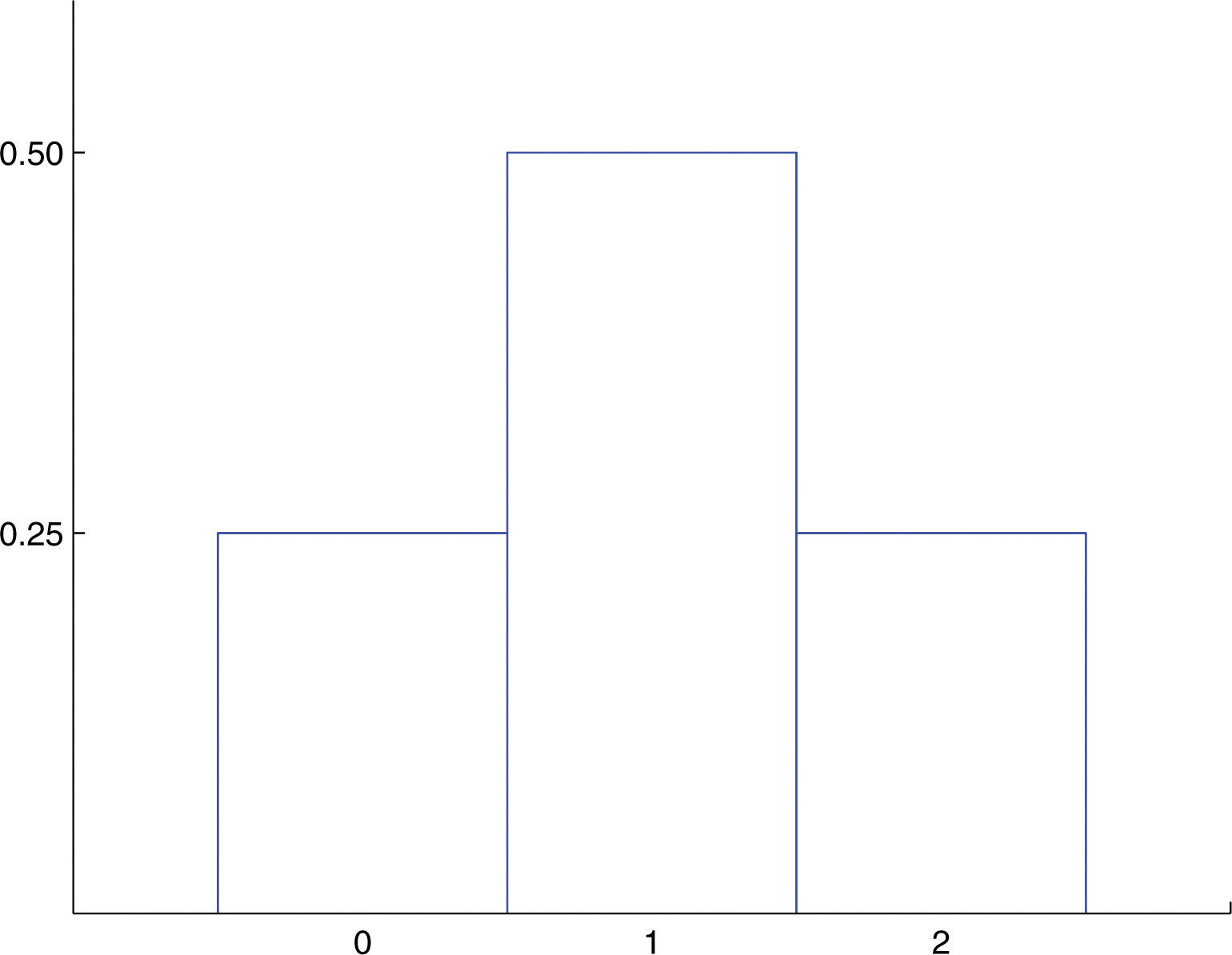
A histogram that graphically illustrates the probability distribution is given in Figure 4.1 "Probability Distribution for Tossing a Fair Coin Twice".
Figure 4.1 Probability Distribution for Tossing a Fair Coin Twice
Example 2
A pair of fair dice is rolled. Let X denote the sum of the number of dots on the top faces.
- Construct the probability distribution of X.
- Find P(X ≥ 9).
- Find the probability that X takes an even value.
Solution:
The sample space of equally likely outcomes is
-
The possible values for X are the numbers 2 through 12. X = 2 is the event {11}, so X = 3 is the event {12,21}, so Continuing this way we obtain the table
This table is the probability distribution of X.
-
The event X ≥ 9 is the union of the mutually exclusive events X = 9, X = 10, X = 11, and X = 12. Thus
-
Before we immediately jump to the conclusion that the probability that X takes an even value must be 0.5, note that X takes six different even values but only five different odd values. We compute
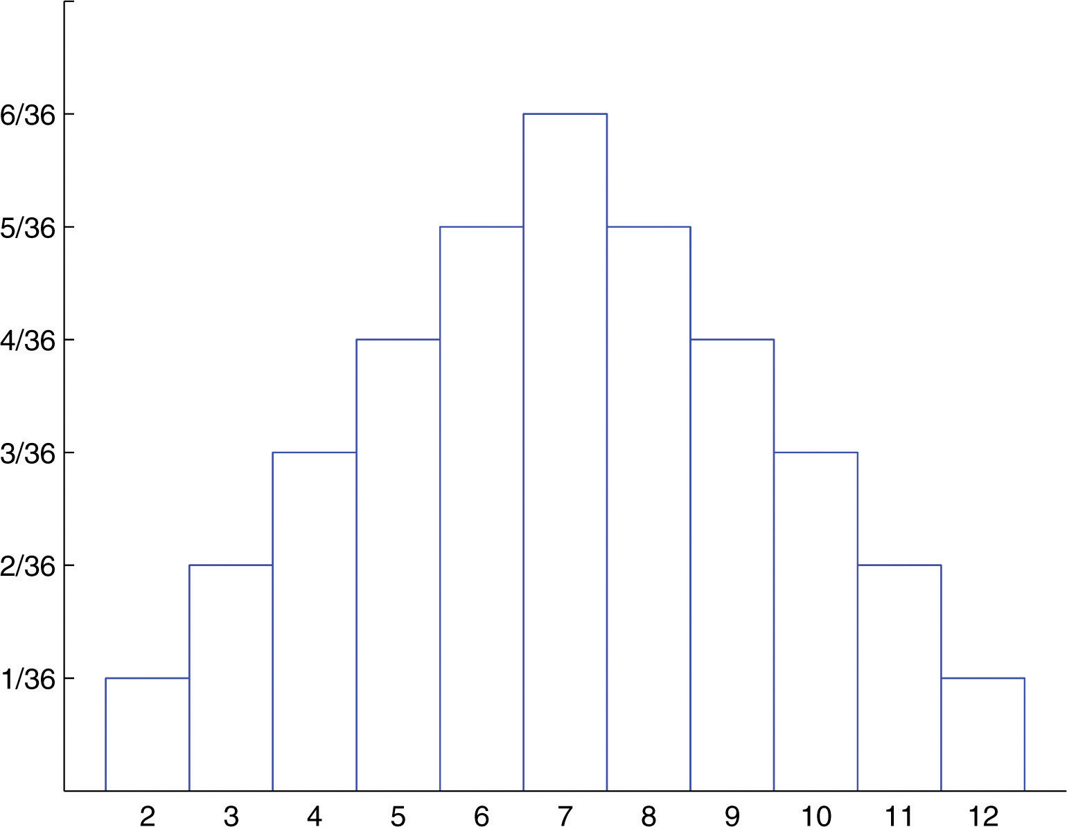
A histogram that graphically illustrates the probability distribution is given in Figure 4.2 "Probability Distribution for Tossing Two Fair Dice".
Figure 4.2 Probability Distribution for Tossing Two Fair Dice
The Mean and Standard Deviation of a Discrete Random Variable
Definition
The meanThe number , measuring its average upon repeated trials. (also called the expected valueIts mean.) of a discrete random variable X is the number
The mean of a random variable may be interpreted as the average of the values assumed by the random variable in repeated trials of the experiment.
Example 3
Find the mean of the discrete random variable X whose probability distribution is
Solution:
The formula in the definition gives
Example 4
A service organization in a large town organizes a raffle each month. One thousand raffle tickets are sold for $1 each. Each has an equal chance of winning. First prize is $300, second prize is $200, and third prize is $100. Let X denote the net gain from the purchase of one ticket.
- Construct the probability distribution of X.
- Find the probability of winning any money in the purchase of one ticket.
- Find the expected value of X, and interpret its meaning.
Solution:
-
If a ticket is selected as the first prize winner, the net gain to the purchaser is the $300 prize less the $1 that was paid for the ticket, hence X = 300 − 1 = 299. There is one such ticket, so P(299) = 0.001. Applying the same “income minus outgo” principle to the second and third prize winners and to the 997 losing tickets yields the probability distribution:
-
Let W denote the event that a ticket is selected to win one of the prizes. Using the table
-
Using the formula in the definition of expected value,
The negative value means that one loses money on the average. In particular, if someone were to buy tickets repeatedly, then although he would win now and then, on average he would lose 40 cents per ticket purchased.
The concept of expected value is also basic to the insurance industry, as the following simplified example illustrates.
Example 5
A life insurance company will sell a $200,000 one-year term life insurance policy to an individual in a particular risk group for a premium of $195. Find the expected value to the company of a single policy if a person in this risk group has a 99.97% chance of surviving one year.
Solution:
Let X denote the net gain to the company from the sale of one such policy. There are two possibilities: the insured person lives the whole year or the insured person dies before the year is up. Applying the “income minus outgo” principle, in the former case the value of X is 195 − 0; in the latter case it is Since the probability in the first case is 0.9997 and in the second case is , the probability distribution for X is:
Therefore
Occasionally (in fact, 3 times in 10,000) the company loses a large amount of money on a policy, but typically it gains $195, which by our computation of works out to a net gain of $135 per policy sold, on average.
Definition
The variance, , of a discrete random variable X is the number
which by algebra is equivalent to the formula
Definition
The standard deviationThe number (also computed using ), measuring its variability under repeated trials., σ, of a discrete random variable X is the square root of its variance, hence is given by the formulas
The variance and standard deviation of a discrete random variable X may be interpreted as measures of the variability of the values assumed by the random variable in repeated trials of the experiment. The units on the standard deviation match those of X.
Example 6
A discrete random variable X has the following probability distribution:
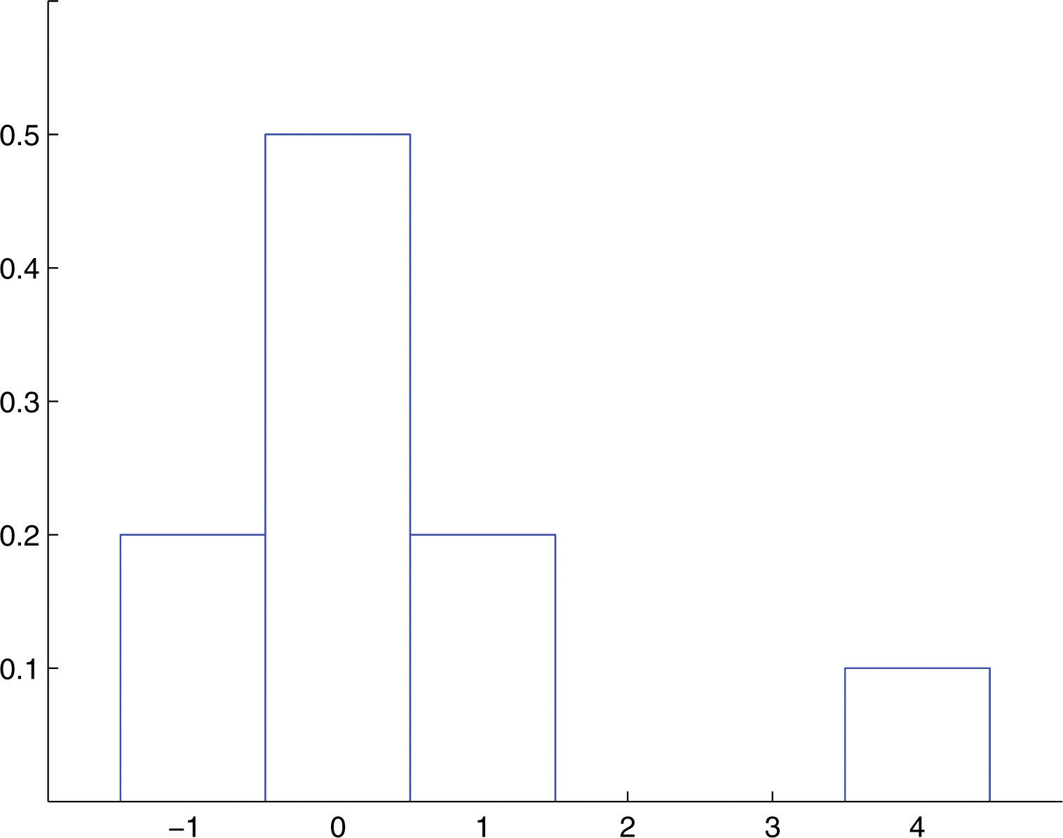
A histogram that graphically illustrates the probability distribution is given in Figure 4.3 "Probability Distribution of a Discrete Random Variable".
Figure 4.3 Probability Distribution of a Discrete Random Variable
Compute each of the following quantities.
- a.
- P(X > 0).
- P(X ≥ 0).
- The mean μ of X.
- The variance of X.
- The standard deviation σ of X.
Solution:
- Since all probabilities must add up to 1,
- Directly from the table,
- From the table,
- From the table,
- Since none of the numbers listed as possible values for X is less than or equal to −2, the event X ≤ −2 is impossible, so P(X ≤ −2) = 0.
-
Using the formula in the definition of μ,
-
Using the formula in the definition of and the value of μ that was just computed,
- Using the result of part (g),
Key Takeaways
- The probability distribution of a discrete random variable X is a listing of each possible value x taken by X along with the probability that X takes that value in one trial of the experiment.
- The mean μ of a discrete random variable X is a number that indicates the average value of X over numerous trials of the experiment. It is computed using the formula
- The variance and standard deviation σ of a discrete random variable X are numbers that indicate the variability of X over numerous trials of the experiment. They may be computed using the formula , taking the square root to obtain σ.
Exercises
-
Determine whether or not the table is a valid probability distribution of a discrete random variable. Explain fully.
-
-
Determine whether or not the table is a valid probability distribution of a discrete random variable. Explain fully.
-
-
A discrete random variable X has the following probability distribution:
Compute each of the following quantities.
- P(X > 80).
- P(X ≤ 80).
- The mean μ of X.
- The variance of X.
- The standard deviation σ of X.
-
A discrete random variable X has the following probability distribution:
Compute each of the following quantities.
- P(X > 18).
- P(X ≤ 18).
- The mean μ of X.
- The variance of X.
- The standard deviation σ of X.
-
If each die in a pair is “loaded” so that one comes up half as often as it should, six comes up half again as often as it should, and the probabilities of the other faces are unaltered, then the probability distribution for the sum X of the number of dots on the top faces when the two are rolled is
Compute each of the following.
- P(X ≥ 7).
- The mean μ of X. (For fair dice this number is 7.)
- The standard deviation σ of X. (For fair dice this number is about 2.415.)
Basic
-
Borachio works in an automotive tire factory. The number X of sound but blemished tires that he produces on a random day has the probability distribution
- Find the probability that Borachio will produce more than three blemished tires tomorrow.
- Find the probability that Borachio will produce at most two blemished tires tomorrow.
- Compute the mean and standard deviation of X. Interpret the mean in the context of the problem.
-
In a hamster breeder's experience the number X of live pups in a litter of a female not over twelve months in age who has not borne a litter in the past six weeks has the probability distribution
- Find the probability that the next litter will produce five to seven live pups.
- Find the probability that the next litter will produce at least six live pups.
- Compute the mean and standard deviation of X. Interpret the mean in the context of the problem.
-
The number X of days in the summer months that a construction crew cannot work because of the weather has the probability distribution
- Find the probability that no more than ten days will be lost next summer.
- Find the probability that from 8 to 12 days will be lost next summer.
- Find the probability that no days at all will be lost next summer.
- Compute the mean and standard deviation of X. Interpret the mean in the context of the problem.
-
Let X denote the number of boys in a randomly selected three-child family. Assuming that boys and girls are equally likely, construct the probability distribution of X.
-
Let X denote the number of times a fair coin lands heads in three tosses. Construct the probability distribution of X.
-
Five thousand lottery tickets are sold for $1 each. One ticket will win $1,000, two tickets will win $500 each, and ten tickets will win $100 each. Let X denote the net gain from the purchase of a randomly selected ticket.
- Construct the probability distribution of X.
- Compute the expected value of X. Interpret its meaning.
- Compute the standard deviation σ of X.
-
Seven thousand lottery tickets are sold for $5 each. One ticket will win $2,000, two tickets will win $750 each, and five tickets will win $100 each. Let X denote the net gain from the purchase of a randomly selected ticket.
- Construct the probability distribution of X.
- Compute the expected value of X. Interpret its meaning.
- Compute the standard deviation σ of X.
-
An insurance company will sell a $90,000 one-year term life insurance policy to an individual in a particular risk group for a premium of $478. Find the expected value to the company of a single policy if a person in this risk group has a 99.62% chance of surviving one year.
-
An insurance company will sell a $10,000 one-year term life insurance policy to an individual in a particular risk group for a premium of $368. Find the expected value to the company of a single policy if a person in this risk group has a 97.25% chance of surviving one year.
-
An insurance company estimates that the probability that an individual in a particular risk group will survive one year is 0.9825. Such a person wishes to buy a $150,000 one-year term life insurance policy. Let C denote how much the insurance company charges such a person for such a policy.
- Construct the probability distribution of X. (Two entries in the table will contain C.)
- Compute the expected value of X.
- Determine the value C must have in order for the company to break even on all such policies (that is, to average a net gain of zero per policy on such policies).
- Determine the value C must have in order for the company to average a net gain of $250 per policy on all such policies.
-
An insurance company estimates that the probability that an individual in a particular risk group will survive one year is 0.99. Such a person wishes to buy a $75,000 one-year term life insurance policy. Let C denote how much the insurance company charges such a person for such a policy.
- Construct the probability distribution of X. (Two entries in the table will contain C.)
- Compute the expected value of X.
- Determine the value C must have in order for the company to break even on all such policies (that is, to average a net gain of zero per policy on such policies).
- Determine the value C must have in order for the company to average a net gain of $150 per policy on all such policies.
-
A roulette wheel has 38 slots. Thirty-six slots are numbered from 1 to 36; half of them are red and half are black. The remaining two slots are numbered 0 and 00 and are green. In a $1 bet on red, the bettor pays $1 to play. If the ball lands in a red slot, he receives back the dollar he bet plus an additional dollar. If the ball does not land on red he loses his dollar. Let X denote the net gain to the bettor on one play of the game.
- Construct the probability distribution of X.
- Compute the expected value of X, and interpret its meaning in the context of the problem.
- Compute the standard deviation of X.
-
A roulette wheel has 38 slots. Thirty-six slots are numbered from 1 to 36; the remaining two slots are numbered 0 and 00. Suppose the “number” 00 is considered not to be even, but the number 0 is still even. In a $1 bet on even, the bettor pays $1 to play. If the ball lands in an even numbered slot, he receives back the dollar he bet plus an additional dollar. If the ball does not land on an even numbered slot, he loses his dollar. Let X denote the net gain to the bettor on one play of the game.
- Construct the probability distribution of X.
- Compute the expected value of X, and explain why this game is not offered in a casino (where 0 is not considered even).
- Compute the standard deviation of X.
-
The time, to the nearest whole minute, that a city bus takes to go from one end of its route to the other has the probability distribution shown. As sometimes happens with probabilities computed as empirical relative frequencies, probabilities in the table add up only to a value other than 1.00 because of round-off error.
- Find the average time the bus takes to drive the length of its route.
- Find the standard deviation of the length of time the bus takes to drive the length of its route.
-
Tybalt receives in the mail an offer to enter a national sweepstakes. The prizes and chances of winning are listed in the offer as: $5 million, one chance in 65 million; $150,000, one chance in 6.5 million; $5,000, one chance in 650,000; and $1,000, one chance in 65,000. If it costs Tybalt 44 cents to mail his entry, what is the expected value of the sweepstakes to him?
Applications
-
The number X of nails in a randomly selected 1-pound box has the probability distribution shown. Find the average number of nails per pound.
-
Three fair dice are rolled at once. Let X denote the number of dice that land with the same number of dots on top as at least one other die. The probability distribution for X is
- Find the missing value u of X.
- Find the missing probability p.
- Compute the mean of X.
- Compute the standard deviation of X.
-
Two fair dice are rolled at once. Let X denote the difference in the number of dots that appear on the top faces of the two dice. Thus for example if a one and a five are rolled, X = 4, and if two sixes are rolled, X = 0.
- Construct the probability distribution for X.
- Compute the mean μ of X.
- Compute the standard deviation σ of X.
-
A fair coin is tossed repeatedly until either it lands heads or a total of five tosses have been made, whichever comes first. Let X denote the number of tosses made.
- Construct the probability distribution for X.
- Compute the mean μ of X.
- Compute the standard deviation σ of X.
-
A manufacturer receives a certain component from a supplier in shipments of 100 units. Two units in each shipment are selected at random and tested. If either one of the units is defective the shipment is rejected. Suppose a shipment has 5 defective units.
- Construct the probability distribution for the number X of defective units in such a sample. (A tree diagram is helpful.)
- Find the probability that such a shipment will be accepted.
-
Shylock enters a local branch bank at 4:30 p.m. every payday, at which time there are always two tellers on duty. The number X of customers in the bank who are either at a teller window or are waiting in a single line for the next available teller has the following probability distribution.
- What number of customers does Shylock most often see in the bank the moment he enters?
- What number of customers waiting in line does Shylock most often see the moment he enters?
- What is the average number of customers who are waiting in line the moment Shylock enters?
-
The owner of a proposed outdoor theater must decide whether to include a cover that will allow shows to be performed in all weather conditions. Based on projected audience sizes and weather conditions, the probability distribution for the revenue X per night if the cover is not installed is
The additional cost of the cover is $410,000. The owner will have it built if this cost can be recovered from the increased revenue the cover affords in the first ten 90-night seasons.
- Compute the mean revenue per night if the cover is not installed.
- Use the answer to (a) to compute the projected total revenue per 90-night season if the cover is not installed.
- Compute the projected total revenue per season when the cover is in place. To do so assume that if the cover were in place the revenue each night of the season would be the same as the revenue on a clear night.
- Using the answers to (b) and (c), decide whether or not the additional cost of the installation of the cover will be recovered from the increased revenue over the first ten years. Will the owner have the cover installed?
Additional Exercises
Answers
-
- no: the sum of the probabilities exceeds 1
- no: a negative probability
- no: the sum of the probabilities is less than 1
-
-
- 0.4
- 0.1
- 0.9
- 79.15
- σ = 1.2359
-
-
- 0.6528
- 0.7153
- μ = 7.8333
- σ = 2.3424
-
-
- 0.79
- 0.60
- μ = 5.8, σ = 1.2570
-
-
-
-
-
- −0.4
- 17.8785
-
-
-
136
-
-
-
- C ≥ 2625
- C ≥ 2875
-
-
-
-
- In many bets the bettor sustains an average loss of about 5.25 cents per bet.
- 0.9986
-
-
-
- 43.54
- 1.2046
-
-
101.02
-
-
-
- 1.9444
- 1.4326
-
-
-
-
- 0.902
-
-
-
- 2523.25
- 227,092.5
- 270,000
- The owner will install the cover.