Chapter 14 General Equilibrium

14.1 Edgeworth Box

The EdgeworthFrancis Edgeworth (1845–1926) introduced a variety of mathematical tools, including calculus, for considering economics and political issues, and was certainly among the first to use advanced mathematics for studying ethical problems. box considers a two-person, two-good “exchange economy.” That is, two people have utility functions of two goods and endowments (initial allocations) of the two goods. The Edgeworth boxA graphical representation of the exchange problem facing participants in a two-good exchange economy. is a graphical representation of the exchange problem facing these people and also permits a straightforward solution to their exchange problem.

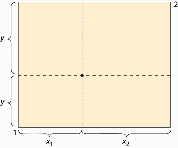
The Edgeworth box is represented in Figure 14.1 "The Edgeworth box". Person 1 is “located” in the lower left (southwest) corner, and Person 2 in the upper right (northeast) corner. The X good is given on the horizontal axis, the Y good on the vertical. The distance between them is the total amount of the good that they have between them. A point in the box gives the allocation of the good—the distance to the lower left to Person 1, the remainder to Person 2. Thus, for the point illustrated, Person 1 obtains (x₁, y₁), and Person 2 obtains (x₂, y₂). The total amount of each good available to the two people will be fixed.

What points are efficient? The economic notion of efficiency is that an allocation is efficient if it is impossible to make one person better off without harming the other person; that is, the only way to improve 1’s utility is to harm 2, and vice versa. Otherwise, if the consumption is inefficient, there is a rearrangement that makes both parties better off, and the parties should prefer such a point. Now, there is no sense of fairness embedded in the notion, and there is an efficient point in which one person gets everything and the other gets nothing. That might be very unfair, but it could still be the case that improving 2 must necessarily harm 1. The allocation is efficient if there is no waste or slack in the system, even if it is wildly unfair. To distinguish this economic notion, it is sometimes called Pareto efficiencyCondition that exists when there is no waste or slack in a system, even if it is wildly unfair..Vilfredo Pareto (1848–1923) was a pioneer in replacing concepts of utility with abstract preferences. His work was later adopted by the economics profession and remains the modern approach.

We can find the Pareto-efficient points by fixing Person 1’s utility and then asking what point, on the indifference isoquant of Person 1, maximizes Person 2’s utility. At that point, any increase in Person 2’s utility must come at the expense of Person 1, and vice versa; that is, the point is Pareto efficient. An example is illustrated in Figure 14.2 "An efficient point".

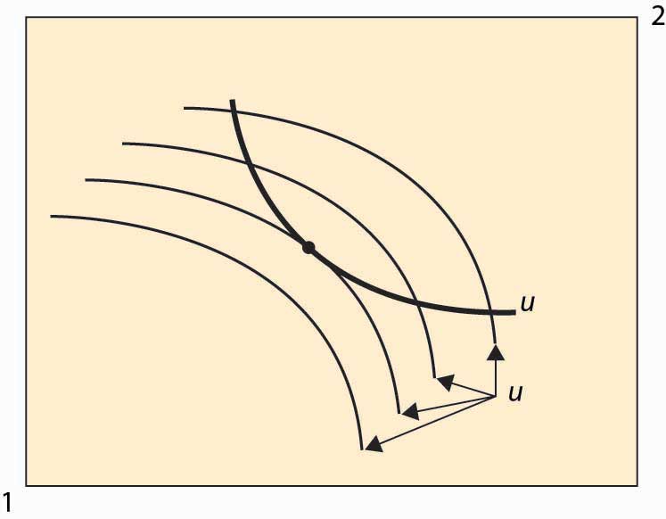
In Figure 14.2 "An efficient point", the isoquant of Person 1 is drawn with a dark, thick line. This utility level is fixed. It acts like the “budget constraint” for Person 2. Note that Person 2’s isoquants face the opposite way because a movement southwest is good for 2, since it gives him more of both goods. Four isoquants are graphed for Person 2, and the highest feasible isoquant, which leaves Person 1 getting the fixed utility, has the Pareto-efficient point illustrated with a large dot. Such points occur at tangencies of the isoquants.

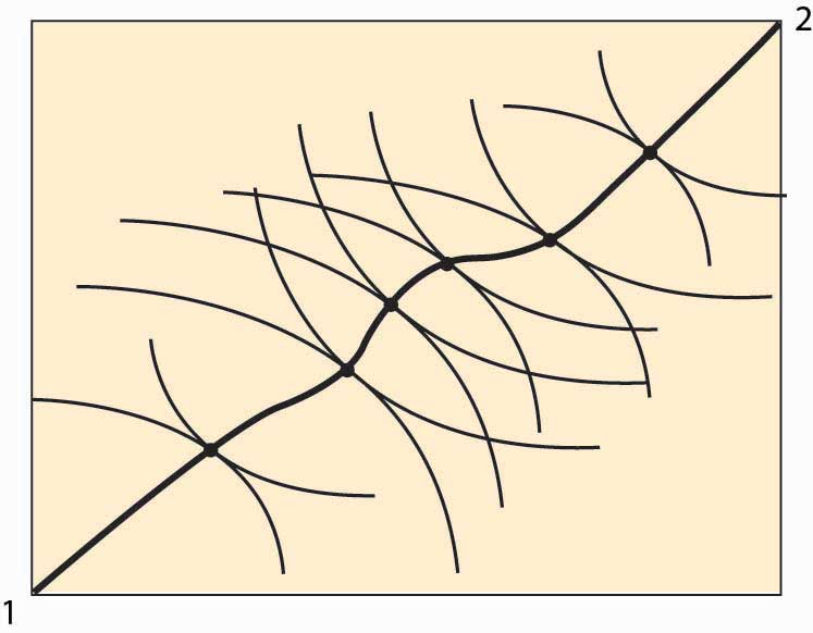
This process of identifying the points that are Pareto efficient can be carried out for every possible utility level for Person 1. What results is the set of Pareto-efficient points, and this set is also known as the contract curveCurve in which every point maximizes one person’s utility given another’s utility.. This is illustrated with the thick line in Figure 14.3 "The contract curve". Every point on this curve maximizes one person’s utility given the other’s utility, and they are characterized by the tangencies in the isoquants.

The contract curve need not have a simple shape, as Figure 14.3 "The contract curve" illustrates. The main properties are that it is increasing and ranges from Person 1 consuming zero of both goods to Person 2 consuming zero of both goods.

Example: Suppose that both people have Cobb-Douglas utility. Let the total endowment of each good be one, so that x₂ = 1 – x₁. Then Person 1’s utility can be written as

u₁ = x^α y^1–αα, and 2’s utility is u₂ = (1 – x)^β (1 – y)^1–β. Then a point is Pareto efficient if

$\frac{\alpha y}{(1-\alpha )x}=\frac{\raisebox{1ex}{$\partial u_1$}\!\left/ \!\raisebox{-1ex}{$\partial x$}\right.}{\raisebox{1ex}{$\partial u_1$}\!\left/ \!\raisebox{-1ex}{$\partial y$}\right.}=\frac{\raisebox{1ex}{$\partial u_2$}\!\left/ \!\raisebox{-1ex}{$\partial x$}\right.}{\raisebox{1ex}{$\partial u_2$}\!\left/ \!\raisebox{-1ex}{$\partial y$}\right.}=\frac{\beta (1-y)}{(1-\beta )(1-x)}\text{.}$

Thus, solving for y, a point is on the contract curve if $y=\frac{(1-\alpha )\beta x}{(1-\beta )\alpha +(\beta -\alpha )x}=\frac{x}{\frac{(1-\beta )\alpha }{(1-\alpha )\beta }+\frac{\beta -\alpha }{(1-\alpha )\beta }x}=\frac{x}{x+\left(\frac{(1-\beta )\alpha }{(1-\alpha )\beta }\right)(1-x)}\text{.}$

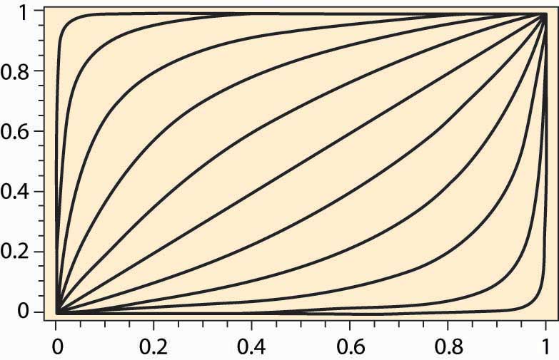
Thus, the contract curve for the Cobb-Douglas case depends on a single parameter $\frac{(1-\beta )\alpha }{(1-\alpha )\beta }\text{.}$ It is graphed for a variety of examples (α and β) in Figure 14.4 "Contract curves with Cobb-Douglas utility".

14.2 Equilibrium With Price System

The contract curve provides the set of efficient points. What point will actually be chosen? Let’s start with an endowment of the goods. An endowment is just a point in the Edgeworth box that represents the initial ownership of both goods for both people. The endowment is marked with a triangle in Figure 14.5 "Individually rational efficient points". Note this point indicates the endowment of both Person 1 and Person 2 because it shows the shares of each.

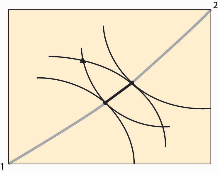
Figure 14.5 "Individually rational efficient points" also shows isoquants for persons 1 and 2 going through the endowment. Note the isoquant for 1 is concave toward the point labeled 1, and the isoquant for 2 is concave toward the point labeled 2. These utility isoquants define a reservation utility level for each person—the utility they could get alone, without exchange. This “no exchange” state is known as autarkyState of no exchange.. There are a variety of efficient points that give these people at least as much as they get under autarky, and those points are along the contract curve but have a darker line.

In Figure 14.5 "Individually rational efficient points", starting at the endowment, the utility of both players is increased by moving in a southeast direction—that is, down and to the right—until the contract curve is reached. This involves Person 1 getting more X (movement to the right) in exchange for giving up some Y (movement down). Thus, we can view the increase in utility as a trade—Person 1 trades some of his Y for some of Person 2’s X.

In principle, any of the darker points on the contract curve, which give both people at least as much as they achieve under autarky, might result from trade. The two people get together and agree on exchange that puts them at any point along this segment of the curve, depending upon the bargaining skills of the players. But there is a particular point, or possibly a set of points, that results from exchange using a price systemSystem that involves a specific price for trading Y for X, and vice versa, that is available to both parties.. A price system involves a specific price for trading Y for X, and vice versa, that is available to both parties. In this figure, prices define a straight line whose slope is the negative of the Y for X price (the X for Y price is the reciprocal).

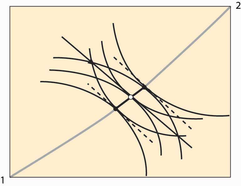
Figure 14.6 "Equilibrium with a price system" illustrates trade with a price system. The O in the center is the point on the contract curve connected to the endowment (triangle) by a straight line (the price line) in such a way that the straight line is tangent to both 1 and 2’s isoquants at the contract curve. This construction means that if each person took the price line as a budget constraint, they would maximize their utility function by choosing the point labeled O.

The fact that a price line exists, that (i) goes through the endowment and (ii) goes through the contract curve at a point tangent to both people’s utility, is relatively easy to show. Consider lines that satisfy property (ii), and let’s see if we can find one that goes through the endowment. Start on the contract curve at the point that maximizes 1’s utility given 2’s reservation utility, and you can easily see that the price line through that point passes above and to the right of the endowment. The similar price line maximizing 2’s utility given 1’s reservation utility passes below and to the left of the endowment. These price lines are illustrated with dotted lines. Thus, by continuity, somewhere in between is a price line that passes through the endowment.

The point labeled O represents an equilibrium of the price system, in so far as supply and demand are equated for both goods. Note, given the endowment and the price through the endowment, both parties maximize utility by going to the O. To see this, it may help to consider a version of the figure that only shows Person 2’s isoquants and the price line.

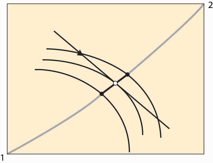
Figure 14.7 "Illustration of price system equilibrium" removes player 1’s isoquants, leaving only player 2’s isoquants and the price line through the endowment. The price line through the endowment is the budget facing each player at that price. Note that, given this budget line, player 2, who gets more as player 1 gets less, maximizes utility at the middle isoquant. That is, taking the price as given, player 2 would choose the O given player 2’s endowment. The logic for player 1 is analogous. This shows that if both players believe that they can buy or sell as much as they like at the trade-off of the price through the O, both will trade to reach the O. This means that if the players accept the price, a balance of supply and demand emerges. In this sense, we have found an equilibrium price.

In the Edgeworth box, we see that, given an endowment, it is possible to reach some Pareto-efficient point using a price system. Moreover, any point on the contract curve arises as an equilibrium of the price system for some endowment. The proof of this proposition is startlingly easy. To show that a particular point on the contract curve is an equilibrium for some endowment, just start with an endowment equal to the point on the contract curve. No trade can occur because the starting point is Pareto efficient—any gain by one party entails a loss by the other.

Furthermore, if a point in the Edgeworth box represents an equilibrium using a price system (that is, if the quantity supplied equals the quantity demanded for both goods), it must be Pareto efficient. At an equilibrium to the price system, each player’s isoquant is tangent to the price line and, hence, tangent to each other. This implies that the equilibrium is Pareto efficient.

Two of the three propositions are known as the first and second welfare theorems of general equilibrium. The first welfare theorem of general equilibriumTheorem that states that any equilibrium of the price system is Pareto efficient. states that any equilibrium of the price system is Pareto efficient. The second welfare theorem of general equilibriumTheorem that states that any Pareto-efficient point is an equilibrium of the price system for some endowment. states that any Pareto-efficient point is an equilibrium of the price system for some endowment. They have been demonstrated by Nobel laureates Kenneth Arrow and Gerard Debreu, for an arbitrary number of people and goods. They also demonstrated the third proposition—that, for any endowment, there exists an equilibrium of the price system with the same high level of generality.

14.3 General Equilibrium

We will illustrate general equilibrium for the case when all consumers have Cobb-Douglas utility in an exchange economyAn economy where the supply of each good is just the total endowment of that good, and there is no production.. An exchange economy is an economy where the supply of each good is just the total endowment of that good, and there is no production. Suppose that there are N people, indexed by n = 1, 2, … , N. There are G goods, indexed by g = 1, 2, … , G. Person n has Cobb-Douglas utility, which we can represent using exponents α(n, g), so that the utility of person n can be represented as ${\displaystyle \prod _{g=1}^{G}x{(n,g)}^{\alpha (n,g)}}\text{,}$ where x(n, g) is person n’s consumption of good g. Assume that α(n, g) ≥ 0 for all n and g, which amounts to assuming that the products are, in fact, goods. Without any loss of generality, we can require ${\displaystyle \sum _{g=1}^G\alpha (n,g)}=1$ for each n. (To see this, note that maximizing the function U is equivalent to maximizing the function U^β for any positive β.)

Let y(n, g) be person n’s endowment of good g. The goal of general equilibrium is to find prices p₁, p₂, … , p_G for the goods in such a way that demand for each good exactly equals supply of the good. The supply of good g is just the sum of the endowments of that good. The prices yield a wealth for person n equal to $W_n={\displaystyle \sum _{g=1}^G{p}_{g}y(n,g)}\text{.}$

We will assume that ${\displaystyle \sum _{n=1}^N\alpha (n,g)y(n,i)}>0$ for every pair of goods g and i. This assumption states that for any pair of goods, there is at least one agent that values good g and has an endowment of good i. The assumption ensures that there is always someone who is willing and able to trade if the price is sufficiently attractive. The assumption is much stronger than necessary but useful for exposition. The assumption also ensures that the endowment of each good is positive.

The Cobb-Douglas utility simplifies the analysis because of a feature that we already encountered in the case of two goods, which holds, in general, that the share of wealth for a consumer n on good g equals the exponent α(n, g). Thus, the total demand for good g is $X_g={\displaystyle \sum _{n=1}^N\frac{\alpha (n,g)W_n}{p_g}}\text{.}$

The equilibrium conditions, then, can be expressed by saying that supply (sum of the endowments) equals demand; or, for each good g, $X_g={\displaystyle \sum _{n=1}^N\frac{\alpha (n,g)W_n}{p_g}}\text{.}$

We can rewrite this expression, provided that p_g > 0 (and it must be, for otherwise demand is infinite), to be $p_g-{\displaystyle \sum _{i=1}^G{p}_i}\frac{{\displaystyle \sum _{n=1}^{N}y(n,i)\alpha (n,g)}}{{\displaystyle \sum _{n=1}^{N}y(n,g)}}=0\text{.}$

Let B be the G × G matrix whose (g, i) term is $b_{gi}=\frac{{\displaystyle \sum _{n=1}^{N}y(n,i)\alpha (n,g)}}{{\displaystyle \sum _{n=1}^{N}y(n,g)}}\text{.}$

Let p be the vector of prices. Then we can write the equilibrium conditions as (I – B) p = 0, where 0 is the zero vector. Thus, for an equilibrium (other than p = 0) to exist, B must have an eigenvalue equal to 1 and a corresponding eigenvector p that is positive in each component. Moreover, if such an eigenvector–eigenvalue pair exists, it is an equilibrium, because demand is equal to supply for each good.

The actual price vector is not completely identified because if p is an equilibrium price vector, then so is any positive scalar times p. Scaling prices doesn’t change the equilibrium because both prices and wealth (which is based on endowments) rise by the scalar factor. Usually economists assign one good to be a numeraire, which means that all other goods are indexed in terms of that good; and the numeraire’s price is artificially set to be 1. We will treat any scaling of a price vector as the same vector.

The relevant theorem is the Perron-Frobenius theoremTheorem that states that if B is a positive matrix (each component positive), then there is an eigenvalue λ > 0 and an associated positive eigenvector p; and, moreover, λ is the largest (in absolute value) eigenvector of B..Oskar Perron (1880–1975) and Georg Frobenius (1849–1917). It states that if B is a positive matrix (each component positive), then there is an eigenvalue λ > 0 and an associated positive eigenvector p; and, moreover, λ is the largest (in absolute value) eigenvector of B.The Perron-Frobenius theorem, as usually stated, only assumes that B is nonnegative and that B is irreducible. It turns out that a strictly positive matrix is irreducible, so this condition is sufficient to invoke the theorem. In addition, we can still apply the theorem even when B has some zeros in it, provided that it is irreducible. Irreducibility means that the economy can’t be divided into two economies, where the people in one economy can’t buy from the people in the second economy because they aren’t endowed with anything that the people in the first economy value. If B is not irreducible, then some people may wind up consuming zero of things they value. This conclusion does most of the work of demonstrating the existence of an equilibrium. The only remaining condition to check is that the eigenvalue is in fact 1, so that (I – B) p = 0.

Suppose that the eigenvalue is λ. Then λp = Bp. Thus for each g,

$$\lambda p_g={\displaystyle \sum _{i=1}^G\frac{{\displaystyle \sum _{n=1}^N\alpha (n,g)y(n,i)}}{{\displaystyle \sum _{m=1}^{N}y(m,g)}}{p}_i}$$

or

$$\lambda p_g{\displaystyle \sum _{m=1}^{N}y(m,g)}={\displaystyle \sum _{i=1}^G{\displaystyle \sum _{n=1}^N\alpha (n,g)y(n,i)}{p}_i}\text{.}$$

Summing both sides over g,

$$\lambda {\displaystyle \sum _{g=1}^G{p}_g{\displaystyle \sum _{m=1}^{N}y(m,g)}}={\displaystyle \sum _{g=1}^G{\displaystyle \sum _{i=1}^G{\displaystyle \sum _{n=1}^N\alpha (n,g)y(n,i)}{p}_i}}$$ $$={\displaystyle \sum _{i=1}^G{\displaystyle \sum _{n=1}^N{\displaystyle \sum _{g=1}^G\alpha (n,g)}y(n,i)}{p}_i}={\displaystyle \sum _{i=1}^G{\displaystyle \sum _{n=1}^{N}y(n,i)}{p}_i}\text{.}$$

Thus, λ = 1 as desired.

The Perron-Frobenius theorem actually provides two more useful conclusions. First, the equilibrium is unique. This is a feature of the Cobb-Douglas utility and does not necessarily occur for other utility functions. Moreover, the equilibrium is readily approximated. Denote by B^t the product of B with itself t times. Then for any positive vector v, $\underset{t\to \infty }{\lim }{B}^{t}v=p\text{.}$ While approximations are very useful for large systems (large numbers of goods), the system can readily be computed exactly with small numbers of goods, even with a large number of individuals. Moreover, the approximation can be interpreted in a potentially useful manner. Let v be a candidate for an equilibrium price vector. Use v to permit people to calculate their wealth, which for person n is $W_n={\displaystyle \sum _{i=1}^G{v}_{i}y(n,i)}\text{.}$ Given the wealth levels, what prices clear the market? Demand for good g is $x_g(v)={\displaystyle \sum _{n=1}^N\alpha (n,g)W_n}={\displaystyle \sum _{i=1}^G{v}_i{\displaystyle \sum _{n=1}^N\alpha (n,g)y(n,i)}}\text{,}$ and the market clears, given the wealth levels, if $p_g=\frac{{\displaystyle \sum _{i=1}^G{v}_i{\displaystyle \sum _{n=1}^N\alpha (n,g)y(n,i)}}}{{\displaystyle \sum _{n=1}^{N}y(n,g)}}\text{,}$ which is equivalent to p = Bv. This defines an iterative process. Start with an arbitrary price vector, compute wealth levels, and then compute the price vector that clears the market for the given wealth levels. Use this price to recalculate the wealth levels, and then compute a new market-clearing price vector for the new wealth levels. This process can be iterated and, in fact, converges to the equilibrium price vector from any starting point.

We finish this section by considering three special cases. If there are two goods, we can let α_n = αα(n, 1), and then conclude that α(n, 2) = 1 – an. Then let $Y_g={\displaystyle \sum _{n=1}^{N}y(n,g)}$ be the endowment of good g. Then the matrix B is $$B=\left(\begin{array}{cc}\frac{1}{Y_1}{\displaystyle \sum _{n=1}^{N}y(n,1)a_n}& \frac{1}{Y_1}{\displaystyle \sum _{n=1}^{N}y(n,2)a_n}\\ \frac{1}{Y_2}{\displaystyle \sum _{n=1}^{N}y(n,1)(1-a_n)}& \frac{1}{Y_2}{\displaystyle \sum _{n=1}^{N}y(n,2)(1-a_n)}\end{array}\right)$$ $$=\left(\begin{array}{cc}\frac{1}{Y_1}{\displaystyle \sum _{n=1}^{N}y(n,1)a_n}& \frac{1}{Y_1}{\displaystyle \sum _{n=1}^{N}y(n,2)a_n}\\ \frac{1}{Y_2}\left(Y_1-{\displaystyle \sum _{n=1}^{N}y(n,1)a_n}\right)& 1-\frac{1}{Y_2}{\displaystyle \sum _{n=1}^{N}y(n,2)a_n}\end{array}\right)\text{.}$$ The relevant eigenvector of B is $$p=\left(\begin{array}{c}{\displaystyle \sum _{n=1}^{N}y(n,2)a_n}\\ {\displaystyle \sum _{n=1}^{N}y(n,1)(1-a_n)}\end{array}\right)\text{.}$$

The overall level of prices is not pinned down—any scalar multiple of p is also an equilibrium price—so the relevant term is the price ratio, which is the price of Good 1 in terms of Good 2, or

$$\frac{p_1}{p_2}=\frac{{\displaystyle \sum _{n=1}^{N}y(n,2)a_n}}{{\displaystyle \sum _{n=1}^{N}y(n,1)(1-a_n)}}\text{.}$$

We can readily see that an increase in the supply of Good 1, or a decrease in the supply of Good 2, decreases the price ratio. An increase in the preference for Good 1 increases the price of Good 1. When people who value Good 1 relatively highly are endowed with a lot of Good 2, the correlation between preference for Good 1, an, and endowment of Good 2 is higher. The higher the correlation, the higher is the price ratio. Intuitively, if the people who have a lot of Good 2 want a lot of Good 1, the price of Good 1 is going to be higher. Similarly, if the people who have a lot of Good 1 want a lot of Good 2, the price of Good 1 is going to be lower. Thus, the correlation between endowments and preferences also matters to the price ratio.

In our second special case, we consider people with the same preferences but who start with different endowments. Hypothesizing identical preferences sets aside the correlation between endowments and preferences found in the two-good case. Since people are the same, α(n, g) = Ag for all n. In this case, $b_{gi}=\frac{{\displaystyle \sum _{n=1}^{N}y(n,i)\alpha (n,g)}}{{\displaystyle \sum _{n=1}^{N}y(n,g)}}=A_g\frac{Y_i}{Y_g}\text{,}$ whereas before $Y_g={\displaystyle \sum _{n=1}^{N}y(n,g)}$ is the total endowment of good g. The matrix B has a special structure, and in this case, $p_g=\frac{A_g}{Y_g}$ is the equilibrium price vector. Prices are proportional to the preference for the good divided by the total endowment for that good.

Now consider a third special case, where no common structure is imposed on preferences, but endowments are proportional to each other; that is, the endowment of person n is a fraction wn of the total endowment. This implies that we can write y(n, g) = w_n Y_g, an equation assumed to hold for all people n and goods g. Note that by construction, ${\displaystyle \sum _{n=1}^N{w}_n}=1\text{,}$ since the value wn represents n’s share of the total endowment. In this case, we have

$$b_{gi}=\frac{{\displaystyle \sum _{n=1}^{N}y(n,i)\alpha (n,g)}}{{\displaystyle \sum _{n=1}^{N}y(n,g)}}=\frac{Y_i}{Y_g}{\displaystyle \sum _{n=1}^N{w}_n\alpha (n,g)}\text{.}$$

These matrices also have a special structure, and it is readily verified that the equilibrium price vector satisfies $p_g=\frac{1}{Y_g}{\displaystyle \sum _{n=1}^N{w}_n\alpha (n,g)}\text{.}$

This formula receives a similar interpretation—the price of good g is the strength of preference for good g, where strength of preference is a wealth-weighted average of the individual preference, divided by the endowment of the good. Such an interpretation is guaranteed by the assumption of Cobb-Douglas preferences, since these imply that individuals spend a constant proportion of their wealth on each good. It also generalizes the conclusion found in the two-good case to more goods, but with the restriction that the correlation is now between wealth and preferences. The special case has the virtue that individual wealth, which is endogenous because it depends on prices, can be readily determined.