13.2 Urban Real Estate Prices

An important point to understand is that the good, in limited supply in cities, is not a physical structure like a house, but the land on which the house sits. The cost of building a house in Los Angeles is quite similar to the cost of building a house in Rochester, New York. The big difference is the price of land. A $1 million house in Los Angeles might be a $400,000 house sitting on a $600,000 parcel of land. The same house in Rochester might be $500,000—a $400,000 house on a $100,000 parcel of land.

Usually, land is what fluctuates in value rather than the price of the house that sits on the land. When a newspaper reports that house prices rose, in fact what rose were land prices, for the price of housing has changed only at a slow pace, reflecting increased wages of house builders and changes in the price of lumber and other inputs. These do change, but historically the changes have been small compared to the price of land.

We can construct a simple model of a city to illustrate the determination of land prices. Suppose the city is constructed on a flat plane. People work at the origin (0, 0). This simplifying assumption is intended to capture the fact that a relatively small, central portion of most cities involves business, with a large area given over to housing. The assumption is extreme, but not unreasonable as a description of some cities.

Suppose commuting times are proportional to distance from the origin. Let c(t) be the cost to the person of a commute of time t, and let the time taken be t = λr, where r is the distance. The function c should reflect both the transportation costs and the value of time lost. The parameter λ accounts for the inverse of the speed in commuting, with a higher λ indicating slower commuting. In addition, we assume that people occupy a constant amount of land. This assumption is clearly wrong empirically, and we will consider making house size a choice variable later.

A person choosing a house priced at p(r), at distance r, thus pays c(λr) + p(r) for the combination of housing and transportation. People will choose the lowest cost alternative. If people have identical preferences about housing and commuting, then house prices p will depend on distance and will be determined by c(λr) + p(r) equal to a constant, so that people are indifferent to the distance from the city’s center—decreased commute time is exactly compensated by increased house prices.

The remaining piece of the model is to figure out the constant. To do this, we need to figure out the area of the city. If the total population is N, and people occupy an area of one per person, then the city size r_max satisfies $N=\pi r_{\max }^2\text{,}$ and thus $r_{\max }=\sqrt{\frac{N}{\pi }}\text{.}$

At the edge of the city, the value of land is given by some other use, like agriculture. From the perspective of the determinant of the city’s prices, this value is approximately constant. As the city takes more land, the change in agricultural land is a very small portion of the total land used for agriculture. Let the value of agricultural land be v per housing unit size. Then the price of housing is p(r_max) = v, because this is the value of land at the edge of the city. This lets us compute the price of all housing in the city:

or

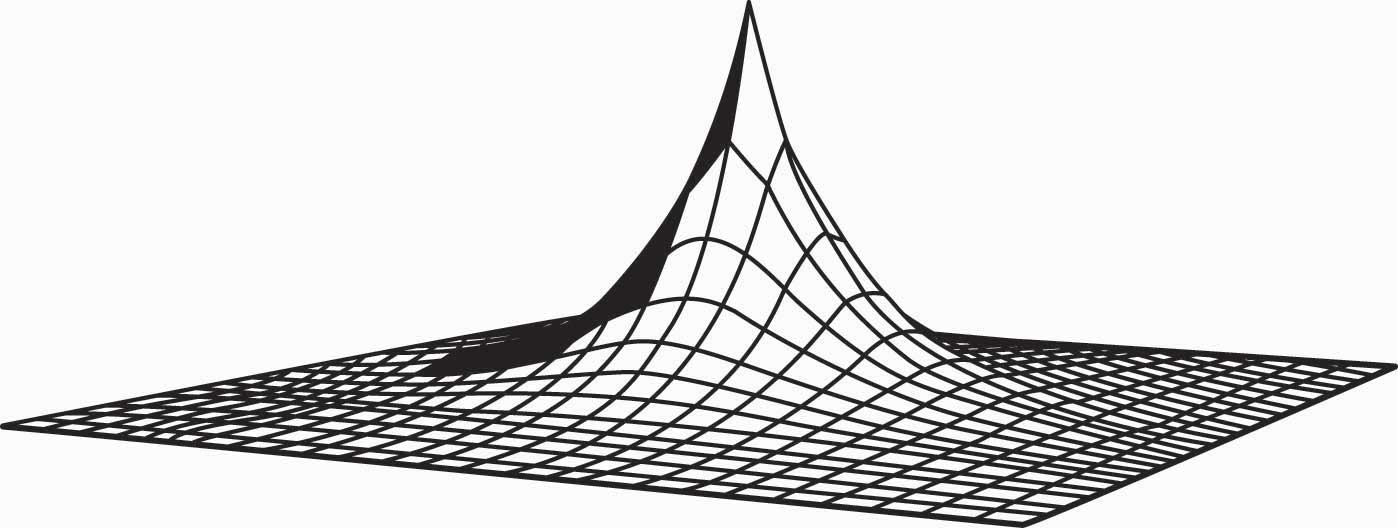
This equation produces housing prices like those illustrated in Figure 13.2 "House price gradient", where the peak is the city’s center. The height of the figure indicates the price of housing.

Figure 13.2 House price gradient

It is straightforward to verify that house prices increase in the population N and the commuting time parameter λ, as one would expect. To quantify the predictions, we consider a city with a population of 1,000,000; a population density of 10,000 per square mile; and an agricultural use value of $6 million per square mile. To translate these assumptions into the model’s structure, first note that a population density of 10,000 per square mile creates a fictitious “unit of measure” of about 52.8 feet, which we’ll call a purlong, so that there is one person per square purlong (2,788 square feet). Then the agricultural value of a property is v = $600 per square purlong. Note that this density requires a city of radius r_max equal to 564 purlongs, which is 5.64 miles.

The only remaining structure left to identify in the model is the commuting cost c. To simplify the calculations, let c be linear. Suppose that the daily cost of commuting is $2 per mile (roundtrip), so that the present value of daily commuting costs in perpetuity is about $10,000 per mile.This amount is based upon 250 working days per year, for an annual cost of about $500 per mile, yielding a present value at 5% interest of $10,000. See Section 11.1 "Present Value". With a time value of $25 per hour and an average speed of 40 mph (1.5 minutes per mile), the time cost is 62.5 cents per minute. Automobile costs (such as gasoline, car depreciation, and insurance) are about 35–40 cents per mile. Thus the total is around $1 per mile, which doubles with roundtrips. This translates into a cost of commuting of $100 per purlong. Thus, we obtain

Thus, the same 2,788-square-foot property at the city’s edge sells for $600 versus $57,000, less than six miles away at the city’s center. With reasonable parameters, this model readily creates dramatic differences in land prices, based purely on commuting time.

As constructed, a quadrupling of population approximately doubles the price of land in the central city. This probably understates the change, since a doubling of the population would likely increase road congestion, increasing λ and further increasing the price of central city real estate.

As presented, the model contains three major unrealistic assumptions. First, everyone lives on an identically sized piece of land. In fact, however, the amount of land used tends to fall as prices rise. At $53 per square foot, most of us buy a lot less land than at 20 cents per square foot. As a practical matter, the reduction of land per capita is accomplished both through smaller housing units and through taller buildings, which produce more housing floor space per acre of land. Second, people have distinct preferences and the disutility of commuting, as well as the value of increased space, varies with the individual. Third, congestion levels are generally endogenous—the more people who live between two points, the greater the traffic density and, consequently, the higher the level of λ. Problems arise with the first two assumptions because of the simplistic nature of consumer preferences embedded in the model, while the third assumption presents an equilibrium issue requiring consideration of transportation choices.

This model can readily be extended to incorporate different types of people, different housing sizes, and endogenous congestion. To illustrate such generalizations, consider making the housing size endogenous. Suppose preferences are represented by the utility function $u=H^{\alpha }-\lambda r-p(r)H\text{,}$ where H is the house size that the person chooses, and r is the distance that he or she chooses. This adaptation of the model reflects two issues. First, the transport cost has been set to be linear in distance for simplicity. Second, the marginal value of housing decreases in the house size, but the value of housing doesn’t depend on distance from the center. For these preferences to make sense, α < 1 (otherwise either zero or an infinite house size emerges). A person with these preferences would optimally choose a house size of $H={\left(\frac{\alpha }{p(r)}\right)}^{\frac{1}{1-\alpha }}\text{,}$ resulting in utility $u*=\left({\alpha }^{\frac{\alpha }{1-\alpha }}-{\alpha }^{\frac{1}{1-\alpha }}\right)p{(r)}^{\frac{-\alpha }{1-\alpha }}-\lambda r\text{.}$ Utility at every location is constant, so ${\left(\frac{{\alpha }^{\frac{\alpha }{1-\alpha }}-{\alpha }^{\frac{1}{1-\alpha }}}{u*+\lambda r}\right)}^{\frac{1-\alpha }{\alpha }}=p(r)\text{.}$

A valuable attribute of the form of the equation for p is that the general form depends on the equilibrium values only through the single number u*. This functional form produces the same qualitative shapes as shown in Figure 13.2 "House price gradient". Using the form, we can solve for the housing size H:

The space in the interval [r, r + Δ] is π(2rΔ + Δ²). In this interval, there are approximately $\frac{\pi (2r\Delta +{\Delta }^2)}{H(r)}=\pi (2r\Delta +{\Delta }^2){\left(\frac{1-\alpha }{\alpha (u*+\lambda r)}\right)}^{\frac{1}{\alpha }}$ people. Thus, the number of people within r_max of the city’s center is ${\displaystyle \underset{0}{\overset{r_{\max }}{\int }}2\pi r{\left(\frac{1-\alpha }{\alpha (u*+\lambda r)}\right)}^{\frac{1}{\alpha }}}dr=N\text{.}$

This equation, when combined with the value of land on the periphery $v=p(r_{\max })={\left(\frac{{\alpha }^{\frac{\alpha }{1-\alpha }}-{\alpha }^{\frac{1}{1-\alpha }}}{u*+\lambda r_{\max }}\right)}^{\frac{1-\alpha }{\alpha }}\text{,}$ jointly determines r_max and u*.

When different people have different preferences, the people with the highest disutility of commuting will tend to live closer to the city’s center. These tend to be people with the highest wages, since one of the costs of commuting is time that could have been spent working.