This is “Isoquants”, section 12.3 from the book Beginning Economic Analysis (v. 1.0). For details on it (including licensing), click here.
For more information on the source of this book, or why it is available for free, please see the project's home page. You can browse or download additional books there. To download a .zip file containing this book to use offline, simply click here.
12.3 Isoquants
Learning Objectives
- What is an isoquant?
- Why does it help to analyze consumer choice?
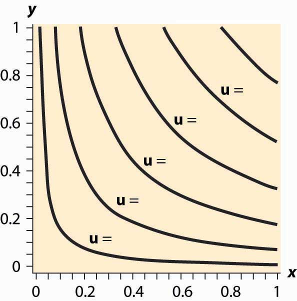
With two goods, we can graphically represent utility by considering the contour map of utility. Utility contours are known as isoquants, meaning “equal quantity,” and are also known as indifference curves, since the consumer is indifferent between points on the line. In other words an indifference curveThe set of goods that produce equal utility; also known as iso-utility curve., also known as an iso-utility curve, is the set of goods that produce equal utility.
We have encountered this idea already in the description of production functions, where the curves represented input mixes that produced a given output. The only difference here is that the output being produced is consumer “utility” instead of a single good or service.
Figure 12.4 Utility isoquants

Figure 12.4 "Utility isoquants" provides an illustration of isoquants, or indifference curves. Each curve represents one level of utility. Higher utilities occur to the northeast, farther away from the origin. As with production isoquants, the slope of the indifference curves has the interpretation of the trade-off between the two goods. The amount of Y that the consumer is willing to give up, in order to obtain an extra bit of X, is the slope of the indifference curve. Formally, the equation defines an indifference curve for the reference utility u0. Differentiating in such a way as to preserve the equality, we obtain the slope of the indifference curve:
or
This slope is known as the marginal rate of substitution and reflects the trade-off, from the consumer’s perspective, between the goods. That is to say, the marginal rate of substitution (of Y for X) is the amount of Y that the consumer is willing to lose in order to obtain an extra unit of X.
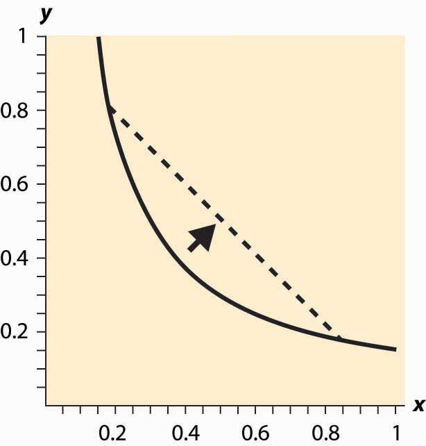
An important assumption concerning isoquants is reflected in the figure: “Midpoints are preferred to extreme points.” Suppose that the consumer is indifferent between (x1, y1) and (x2, y2); that is, u(x1, y1) = u(x2, y2). Then we can say that preferences are convex if any point on the line segment connecting (x1, y1) and (x2, y2) is at least as good as the extremes. Formally, a point on the line segment connecting (x1, y1) and (x2, y2) comes in the form (αx1 + (1 – α) x2, αy1 + (1 – α) y2), for α between zero and one. This is also known as a “convex combination” between the two points. When α is zero, the segment starts at (x2, y2) and proceeds in a linear fashion to (x1, y1) at α = 1. Preferences are convex if, for any α between 0 and 1, u(x1, y1) = u(x2, y2) implies u(αx1 + (1 – α) x2, (y1 + (1 – α) y2) ≥ u(x1, y1).
This property is illustrated in Figure 12.5 "Convex preferences". The line segment that connects two points on the indifference curve lies to the northeast of the indifference curve, which means that the line segment involves strictly more consumption of both goods than some points on the indifference curve. In other words, it is preferred to the indifference curve. Convex preferences mean that a consumer prefers a mix to any two equally valuable extremes. Thus, if the consumer likes black coffee and also likes drinking milk, then the consumer prefers some of each—not necessarily mixed—to only drinking coffee or only drinking milk. This sounds more reasonable if you think of the consumer’s choices on a monthly basis. If you like drinking 60 cups of coffee and no milk per month as much as you like drinking 30 glasses of milk and no coffee, convex preferences entail preferring 30 cups of coffee and 15 glasses of milk to either extreme.
Figure 12.5 Convex preferences

How does a consumer choose which bundle to select? The consumer is faced with the problem of maximizing u(x, y) subject to
We can derive the solution to the consumer’s problem as follows. First, “solve” the budget constraint for y, to obtain If Y is a good, this constraint will be satisfied with equality, and all of the money will be spent. Thus, we can write the consumer’s utility as
The first-order condition for this problem, maximizing it over x, has
This can be rearranged to obtain the marginal rate of substitution (MRS):
The marginal rate of substitution (MRS)The amount extra of one good needed to make up for a decrease in another good, staying on an indifference curve. is the extra amount of one good needed to make up for a decrease in another good, staying on an indifference curve
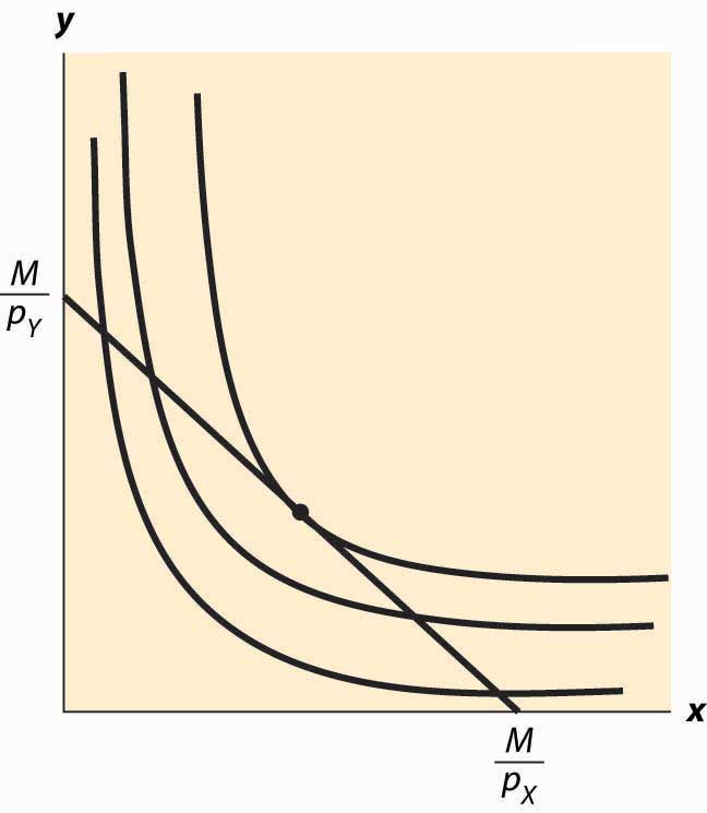
The first-order condition requires that the slope of the indifference curve equals the slope of the budget line; that is, there is a tangency between the indifference curve and the budget line. This is illustrated in Figure 12.6 "Graphical utility maximization". Three indifference curves are drawn, two of which intersect the budget line but are not tangent. At these intersections, it is possible to increase utility by moving “toward the center,” until the highest of the three indifference curves is reached. At this point, further increases in utility are not feasible, because there is no intersection between the set of bundles that produce a strictly higher utility and the budget set. Thus, the large black dot is the bundle that produces the highest utility for the consumer.
It will later prove useful to also state the second-order condition, although we won’t use this condition now:
Note that the vector is the gradient of u, and the gradient points in the direction of steepest ascent of the function u. Second, the equation that characterizes the optimum,
Figure 12.6 Graphical utility maximization

where • is the “dot product” that multiplies the components of vectors and then adds them, says that the vectors (u1, u2) and (–pY, pX) are perpendicular and, hence, that the rate of steepest ascent of the utility function is perpendicular to the budget line.
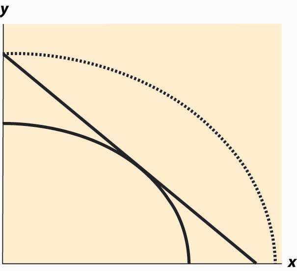
When does this tangency approach fail to solve the consumer’s problem? There are three ways that it can fail. First, the utility might not be differentiable. We will set aside this kind of failure with the remark that fixing points of nondifferentiability is mathematically challenging but doesn’t lead to significant alterations in the theory. The second failure is that a tangency doesn’t maximize utility. Figure 12.7 "“Concave” preferences: Prefer boundaries" illustrates this case. Here there is a tangency, but it doesn’t maximize utility. In Figure 12.7 "“Concave” preferences: Prefer boundaries" , the dotted indifference curve maximizes utility given the budget constraint (straight line). This is exactly the kind of failure that is ruled out by convex preferences. In Figure 12.7 "“Concave” preferences: Prefer boundaries", preferences are not convex because, if we connect two points on the indifference curves and look at a convex combination, we get something less preferred, with lower utility—not more preferred as convex preferences would require.
Figure 12.7 “Concave” preferences: Prefer boundaries

The third failure is more fundamental: The derivative might fail to be zero because we’ve hit the boundary of x = 0 or y = 0. This is a fundamental problem because, in fact, there are many goods that we do buy zero of, so zeros for some goods are not uncommon solutions to the problem of maximizing utility. We will take this problem up in a separate section, but we already have a major tool to deal with it: convex preferences. As we shall see, convex preferences ensure that the consumer’s maximization problem is “well behaved.”
Key Takeaways
- Isoquants, meaning “equal quantity,” are also known as indifference curves and represent sets of points holding utility constant. They are analogous to production isoquants.
- Preferences are said to be convex if any point on the line segment connecting a pair of points with equal utility is preferred to the endpoints. This means that whenever the consumer is indifferent between two points, he or she prefers a mix of the two.
- The first-order conditions for the maximizing utility involve equating the marginal rate of substitution and the price ratio.
- At the maximum, the rate of steepest ascent of the utility function is perpendicular to the budget line.
- There are two main ways that the first-order conditions fail to characterize the optimum: the consumer doesn’t have convex preferences, or the optimum involves a zero consumption of one or more goods.


