9.2 Production Functions

The firm transforms inputs into outputs. For example, a bakery takes inputs like flour, water, yeast, labor, and heat and makes loaves of bread. An earth moving company combines capital equipment, ranging from shovels to bulldozers with labor in order to digs holes. A computer manufacturer buys parts “off-the-shelf” like disk drives and memory, with cases and keyboards, and combines them with labor to produce computers. Starbucks takes coffee beans, water, some capital equipment, and labor to brew coffee.

Many firms produce several outputs. However, we can view a firm that is producing multiple outputs as employing distinct production processes. Hence, it is useful to begin by considering a firm that produces only one output. We can describe this firm as buying an amount x₁ of the first input, x₂ of the second input, and so on (we’ll use xn to denote the last input), and producing a quantity of the output. The production function that describes this process is given by y = f(x₁, x₂, … , xn).

The production functionThe mapping from inputs to an output or outputs. is the mapping from inputs to an output or outputs.

For the most part we will focus on two inputs in this section, although the analyses with more than inputs is “straightforward.”

Example: The Cobb-Douglas production functionA production function that is the product of each input, x, raised to a given power. is the product of each input, x, raised to a given power. It takes the form $f(x_1,x_2,\mathrm{\dots },x_n)=a_0{x}_1^{a_1}{x}_2^{a_2}\mathrm{\dots }{x}_n^{a_n}\text{.}$

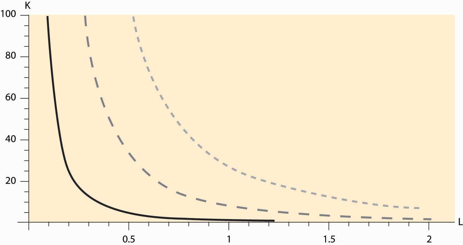
The constants a₁ through an are typically positive numbers less than one. For example, with two goods, capital K and labor L, the Cobb-Douglas function becomes a₀K^aL^b. We will use this example frequently. It is illustrated, for a₀ = 1, a = 1/3, and b = 2/3, in Figure 9.1 "Cobb-Douglas isoquants".

Figure 9.1 Cobb-Douglas isoquants

Figure 9.1 "Cobb-Douglas isoquants" illustrates three isoquants for the Cobb-Douglas production function. An isoquantCurves that describe all the combinations of inputs that produce the same level of output., which means “equal quantity,” is a curve that describes all the combinations of inputs that produce the same level of output. In this case, given a = 1/3 and b = 2/3, we can solve y = K^aL^b for K to obtain K = y³ L^-2. Thus, K = L^-2 gives the combinations of inputs yielding an output of 1, which is denoted by the dark, solid line in Figure 9.1 "Cobb-Douglas isoquants" The middle, gray dashed line represents an output of 2, and the dotted light-gray line represents an output of 3. Isoquants are familiar contour plots used, for example, to show the height of terrain or temperature on a map. Temperature isoquants are, not surprisingly, called isotherms.

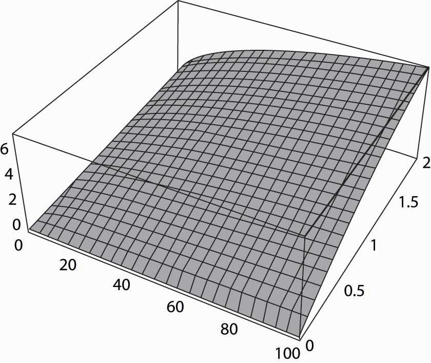
Figure 9.2 The production function

Isoquants provide a natural way of looking at production functions and are a bit more useful to examine than three-dimensional plots like the one provided in Figure 9.2 "The production function".

The fixed-proportions production function comes in the form $f(x_1,x_2,\mathrm{\dots },x_n)=Min\{a_1{x}_1,a_2{x}_2,\mathrm{\dots },a_n{x}_n\}\text{.}$

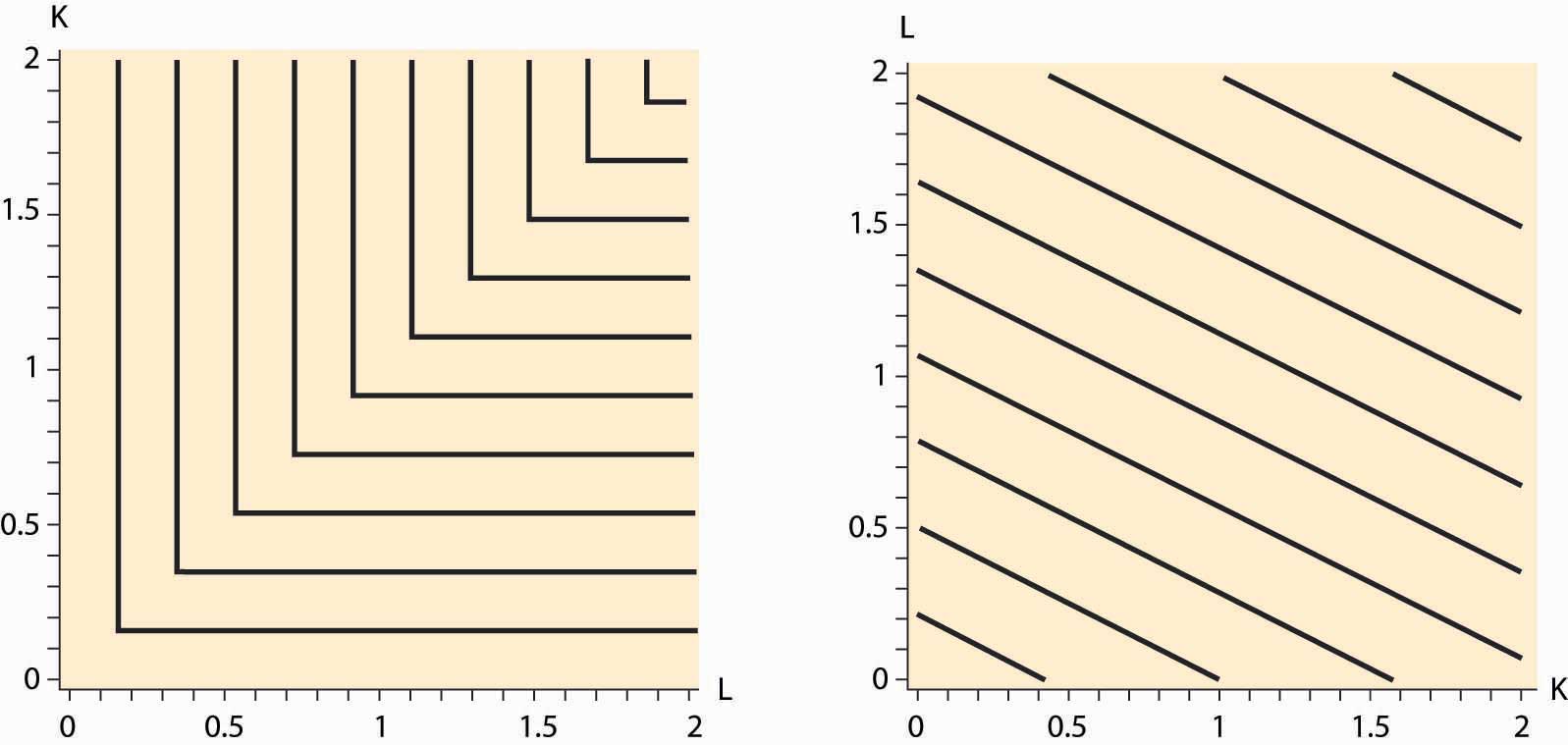
The fixed-proportions production functionA production function that requires inputs be used in fixed proportions to produce output. is a production function that requires inputs be used in fixed proportions to produce output. It has the property that adding more units of one input in isolation does not necessarily increase the quantity produced. For example, the productive value of having more than one shovel per worker is pretty low, so that shovels and diggers are reasonably modeled as producing holes using a fixed-proportions production function. Moreover, without a shovel or other digging implement like a backhoe, a barehanded worker is able to dig so little that he is virtually useless. Ultimately, the size of the holes is determined by min {number of shovels, number of diggers}. Figure 9.3 "Fixed-proportions and perfect substitutes" illustrates the isoquants for fixed proportions. As we will see, fixed proportions make the inputs “perfect complements.”

Figure 9.3 Fixed-proportions and perfect substitutes

Two inputs K and L are perfect substitutes in a production function f if they enter as a sum; so that f(K, L, x₃, … , xn) = g(K + cL, x₃, … , xn) for a constant c. Another way of thinking of perfect substitutesTwo goods that can be substituted for each other at a constant rate while maintaining the same output level. is that they are two goods that can be substituted for each other at a constant rate while maintaining the same output level. With an appropriate scaling of the units of one of the variables, all that matters is the sum of the two variables, not their individual values. In this case, the isoquants are straight lines that are parallel to each other, as illustrated in Figure 9.3 "Fixed-proportions and perfect substitutes".

The marginal productThe derivative of the production function with respect to an input. of an input is just the derivative of the production function with respect to that input.This is a partial derivative, since it holds the other inputs fixed. Partial derivatives are denoted with the symbol δ. An important property of marginal product is that it may be affected by the level of other inputs employed. For example, in the Cobb-Douglas case with two inputsThe symbol α is the Greek letter “alpha.” The symbol β is the Greek letter “beta.” These are the first two letters of the Greek alphabet, and the word alphabet itself originates from these two letters. and for constant A,

the marginal product of capital is

If α and β are between zero and one (the usual case), then the marginal product of capital is increasing in the amount of labor, and it is decreasing in the amount of capital employed. For example, an extra computer is very productive when there are many workers and a few computers, but it is not so productive where there are many computers and a few people to operate them.

The value of the marginal productThe marginal product times the price of the output. of an input is the marginal product times the price of the output. If the value of the marginal product of an input exceeds the cost of that input, it is profitable to use more of the input.

Some inputs are easier to change than others. It can take 5 years or more to obtain new passenger aircraft, and 4 years to build an electricity generation facility or a pulp and paper mill. Very skilled labor such as experienced engineers, animators, and patent attorneys are often hard to find and challenging to hire. It usually requires one to spend 3 to 5 years to hire even a small number of academic economists. On the other hand, it is possible to buy shovels, telephones, and computers or to hire a variety of temporary workers rapidly, in a day or two. Moreover, additional hours of work can be obtained from an existing labor force simply by enlisting them to work “overtime,” at least on a temporary basis. The amount of water or electricity that a production facility uses can be varied each second. A dishwasher at a restaurant may easily use extra water one evening to wash dishes if required. An employer who starts the morning with a few workers can obtain additional labor for the evening by paying existing workers overtime for their hours of work. It will likely take a few days or more to hire additional waiters and waitresses, and perhaps several days to hire a skilled chef. You can typically buy more ingredients, plates, and silverware in one day, whereas arranging for a larger space may take a month or longer.

The fact that some inputs can be varied more rapidly than others leads to the notions of the long run and the short run. In the short run, only some inputs can be adjusted, while in the long run all inputs can be adjusted. Traditionally, economists viewed labor as quickly adjustable and capital equipment as more difficult to adjust. That is certainly right for airlines—obtaining new aircraft is a very slow process—for large complex factories, and for relatively low-skilled, and hence substitutable, labor. On the other hand, obtaining workers with unusual skills is a slower process than obtaining warehouse or office space. Generally speaking, the long-run inputs are those that are expensive to adjust quickly, while the short-run factors can be adjusted in a relatively short time frame. What factors belong in which category is dependent on the context or application under consideration.