This is “Trade”, chapter 6 from the book Beginning Economic Analysis (v. 1.0). For details on it (including licensing), click here.
For more information on the source of this book, or why it is available for free, please see the project's home page. You can browse or download additional books there. To download a .zip file containing this book to use offline, simply click here.


Chapter 6 Trade
Supply and demand offers one approach to understanding trade, and it represents the most important and powerful concept in the toolbox of economists. However, for some issues, especially those of international trade, another related tool is very useful: the production possibilities frontier. Analysis using the production possibilities frontier was made famous by the “guns and butter” discussions of World War II. From an economic perspective, there is a trade-off between guns and butter—if a society wants more guns, it must give up something, and one thing to give up is butter. While the notion of getting more guns might lead to less butter often seems mysterious, butter is, after all, made with cows, and indirectly with land and hay. But the manufacture of butter also involves steel containers, tractors to turn the soil, transportation equipment, and labor, all of which either can be directly used (steel, labor) or require inputs that could be used (tractors, transportation) to manufacture guns. From a production standpoint, more guns entail less butter (or other things).
6.1 Production Possibilities Frontier
Learning Objective
- What can we produce, and how does that relate to cost?
Formally, the set of production possibilitiesThe collection of feasible outputs of an individual, group or society, or country. is the collection of “feasible outputs” of an individual, group or society, or country. You could spend your time cleaning your apartment, or you could study. The more time you devote to studying, the higher your grades will be, but the dirtier your apartment will be. This is illustrated, for a hypothetical student, in Figure 6.1 "The production possibilities frontier".
The production possibilities set embodies the feasible alternatives. If you spend all your time studying, you could obtain a 4.0 (perfect) grade point average (GPA). Spending an hour cleaning reduces the GPA, but not by much; the second hour reduces it by a bit more, and so on.
The boundary of the production possibilities set is known as the production possibilities frontierThe boundary of the production possibilities set.. This is the most important part of the production possibilities set because, at any point strictly inside the production possibilities set, it is possible to have more of everything, and usually we would choose to have more.To be clear, we are considering an example with two goods: cleanliness and GPA. Generally there are lots of activities, like sleeping, eating, teeth brushing, and so on; the production possibilities frontier encompasses all of these goods. Spending all your time sleeping, studying, and cleaning would still represent a point on a three-dimensional frontier. The slope of the production possibilities frontier reflects opportunity cost because it describes what must be given up in order to acquire more of a good. Thus, to get a cleaner apartment, more time or capital, or both, must be spent on cleaning, which reduces the amount of other goods and services that can be had. For the two-good case in Figure 6.1 "The production possibilities frontier", diverting time to cleaning reduces studying, which lowers the GPA. The slope dictates how much lost GPA there is for each unit of cleaning.
Figure 6.1 The production possibilities frontier
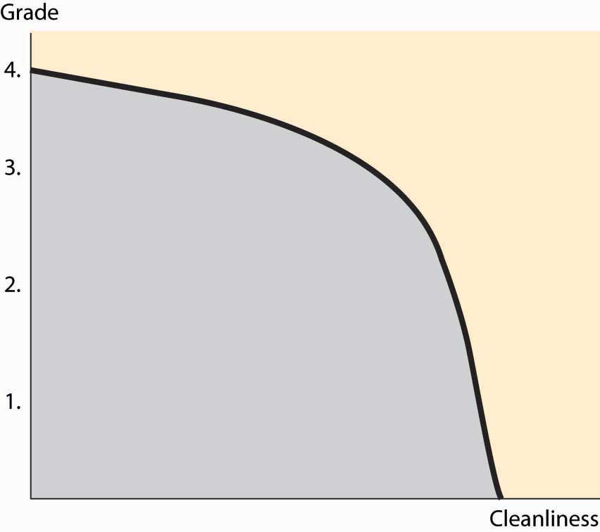
One important feature of production possibilities frontiers is illustrated in Figure 6.1 "The production possibilities frontier": They are concave toward the origin. While this feature need not be universally true, it is a common feature, and there is a reason for it that we can see in the application. If you are only going to spend an hour studying, you spend that hour doing the most important studying that can be done in an hour, and thus get a substantial improvement in grades for the hour’s work. The second hour of studying produces less value than the first, and the third hour less than the second. Thus, spending more on something reduces the per-unit value produced. This is the principle of Diminishing marginal returnsThe principle that spending more on something reduces the per-unit value produced.. Diminishing marginal returns are like picking apples. If you are only going to pick apples for a few minutes, you don’t need a ladder because the fruit is low on the tree; the more time spent, the fewer apples per hour you will pick.
Consider two people, Ann and Bob, getting ready for a party. One is cutting up vegetables; the other is making hors d’oeuvres. Ann can cut up 2 ounces of vegetables per minute, or make one hors d’oeuvre in a minute. Bob, somewhat inept with a knife, can cut up 1 ounce of vegetables per minute, or make 2 hors d’oeuvres per minute. Ann and Bob’s production possibilities frontiers are illustrated in Figure 6.2 "Two production possibilities frontiers", given that they have an hour to work.
Since Ann can produce 2 ounces of chopped vegetables in a minute, if she spends her entire hour on vegetables, she can produce 120 ounces. Similarly, if she devotes all her time to hors d’oeuvres, she produces 60 of them. The constant translation between the two means that her production possibilities frontier is a straight line, which is illustrated on the left side of Figure 6.2 "Two production possibilities frontiers". Bob’s is the reverse—he produces 60 ounces of vegetables or 120 hors d’oeuvres, or something on the line in between.
Figure 6.2 Two production possibilities frontiers
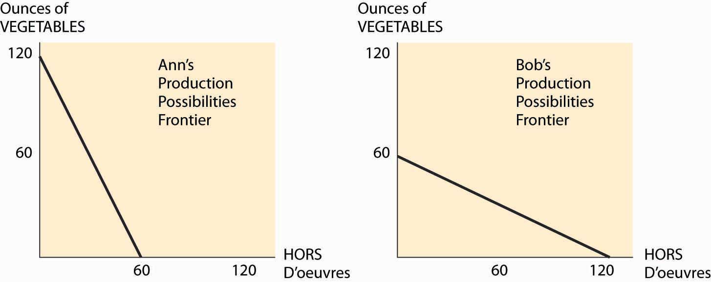
For Ann, the opportunity cost of an ounce of vegetables is half of one hors d’oeuvre—to get one extra ounce of vegetables, she must spend 30 extra seconds on vegetables. Similarly, the cost of one hors d’oeuvre for Ann is 2 ounces of vegetables. Bob’s costs are the inverse of Ann’s—an ounce of vegetables costs him two hors d’oeuvres.
Figure 6.3 Joint PPF
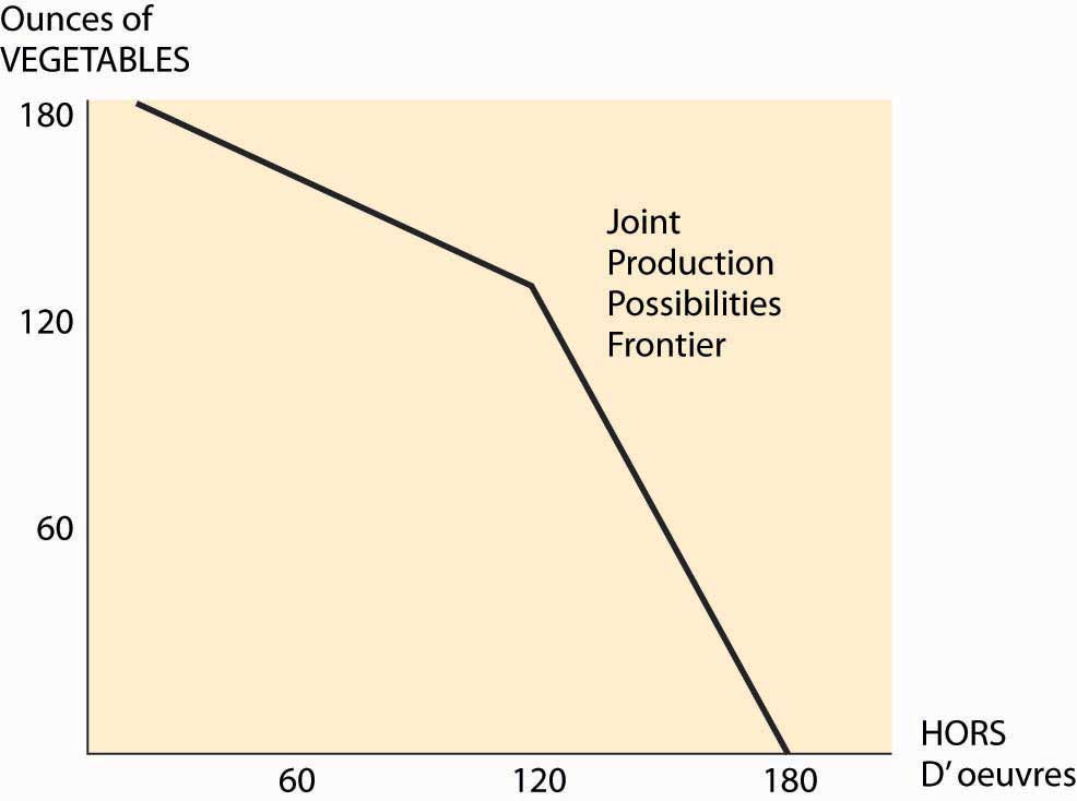
What can Bob and Ann accomplish together? The important insight is that they should use the low-cost person in the manufacture of each good, when possible. This means that if fewer than 120 ounces of vegetables will be made, Ann makes them all. Similarly, if fewer than 120 hors d’oeuvres are made, Bob makes them all. This gives a joint production possibilities frontier as illustrated in Figure 6.3 "Joint PPF". Together, they can make 180 of one and none of the other. If Bob makes only hors d’oeuvres, and Ann makes only chopped vegetables, they will have 120 of each. With fewer than 120 ounces of vegetables, the opportunity cost of vegetables is Ann’s, and is thus half an hors d’oeuvre; but if more than 120 are needed, then the opportunity cost jumps to two.
Now change the hypothetical slightly. Suppose that Bob and Ann are putting on separate dinner parties, each of which will feature chopped vegetables and hors d’oeuvres in equal portions. By herself, Ann can only produce 40 ounces of vegetables and 40 hors d’oeuvres if she must produce equal portions. She accomplishes this by spending 20 minutes on vegetables and 40 minutes on hors d’oeuvres. Similarly, Bob can produce 40 of each, but by using the reverse allocation of time.
By working together, they can collectively have more of both goods. Ann specializes in producing vegetables, and Bob specializes in producing hors d’oeuvres. This yields 120 units of each, which they can split equally to have 60 of each. By specializing in the activity in which they have lower cost, Bob and Ann can jointly produce more of each good.
Moreover, Bob and Ann can accomplish this by trading. At a “one for one” price, Bob can produce 120 hors d’oeuvres, and trade 60 of them for 60 ounces of vegetables. This is better than producing the vegetables himself, which netted him only 40 of each. Similarly, Ann produces 120 ounces of vegetables and trades 60 of them for 60 hors d’oeuvres. This trading makes them both better off.
The gains from specialization are potentially enormous. The grandfather of economics, Adam Smith, wrote about specialization in the manufacture of pins:
One man draws out the wire; another straights it; a third cuts it; a fourth points it; a fifth grinds it at the top for receiving the head; to make the head requires two or three distinct operations; to put it on is a peculiar business; to whiten the pins is another; it is even a trade by itself to put them into the paper; and the important business of making a pin is, in this manner, divided into about eighteen distinct operations, which, in some manufactories, are all performed by distinct hands, though in others the same man will sometimes perform two or three of them.Adam Smith, An Inquiry into the Nature and Causes of the Wealth of Nations, originally published in 1776, released by the Gutenberg project, 2002.
Smith goes on to say that skilled individuals could produce at most 20 pins per day acting alone; but that, with specialization, 10 people could produce 48,000 pins per day, 240 times as many pins per capita.
Key Takeaways
- The production possibilities set is the collection of “feasible outputs” of an individual or group.
- The boundary of the production possibilities set is known as the production possibilities frontier.
- The principle of diminishing marginal returns implies that the production possibilities frontier is concave toward the origin, which is equivalent to increasing opportunity cost.
- Efficiencies created by specialization create the potential for gains from trade.
Exercises
- The Manning Company has two factories, one that makes roof trusses and one that makes cabinets. With m workers, the roof factory produces trusses per day. With n workers, the cabinet plant produces The Manning Company has 400 workers to use in the two factories. Graph the production possibilities frontier. (Hint: Let T be the number of trusses produced. How many workers are used to make trusses?)
- Alarm & Tint, Inc., has 10 workers working a total of 400 hours per week. Tinting takes 2 hours per car. Alarm installation is complicated, however, and performing A alarm installations requires A2 hours of labor. Graph Alarm & Tint’s production possibilities frontier for a week.
-
Consider two consumers and two goods, x and y. Consumer 1 has utility u1(x1, y1) = x1 + y1 and consumer 2 has utility u2(x2, y2) = min {x2, y2}. Consumer 1 has an endowment of (1, 1/2) and consumer 2’s endowment is (0, 1/2).
- Draw the Edgeworth box for this economy.
- Find the contract curve and the individually rational part of it. (You should describe these in writing and highlight them in the Edgeworth box.)
- Find the prices that support an equilibrium of the system and the final allocation of goods under those prices.
For Questions 4 to 7, consider an orange juice factory that uses, as inputs, oranges and workers. If the factory uses x pounds of oranges and y workers per hour, it produces gallons of orange juice; T = 20x0.25y0.5.
- Suppose oranges cost $1 and workers cost $10. What relative proportion of oranges and workers should the factory use?
- Suppose a gallon of orange juice sells for $1. How many units should be sold, and what is the input mix to be used? What is the profit?
- Generalize the previous exercise for a price of p dollars per gallon of orange juice.
- What is the supply elasticity?
6.2 Comparative and Absolute Advantage
Learning Objectives
- Who can produce more?
- How does that relate to cost?
- Can a nation be cheaper on all things?
Ann produces chopped vegetables because her opportunity cost of producing vegetables, at half of one hors d’oeuvre, is lower than Bob’s. When one good has a lower opportunity cost over another, it is said to have a comparative advantageCondition that exists when one good has a lower opportunity cost over another.. That is, Ann gives up less to produce chopped vegetables than Bob, so in comparison to hors d’oeuvres, she has an advantage in the production of vegetables. Since the cost of one good is the amount of another good forgone, a comparative advantage in one good implies a comparative disadvantageCondition that exists when one good has a higher opportunity cost over another.—a higher opportunity cost—in another. If you are better at producing butter, you are necessarily worse at something else—and, in particular, the thing you give up less of to get more butter.
To illustrate this point, let’s consider another party planner. Charlie can produce one hors d’oeuvre or 1 ounce of chopped vegetables per minute. His production is strictly less than Ann’s; that is, his production possibilities frontier lies inside of Ann’s. However, he has a comparative advantage over Ann in the production of hors d’oeuvres because he gives up only 1 ounce of vegetables to produce an hors d’oeuvre, while Ann must give up 2 ounces of vegetables. Thus, Ann and Charlie can still benefit from trade if Bob isn’t around.
When one production possibilities frontier lies outside another, the larger is said to have an absolute advantageCondition that exists when one production possibilities frontier can produce more of all goods than another.—it can produce more of all goods than the smaller. In this case, Ann has an absolute advantage over Charlie—she can, by herself, have more—but not over Bob. Bob has an absolute advantage over Charlie, too; but again, not over Ann.
Diminishing marginal returns implies that the more of a good that a person produces, the higher the cost is (in terms of the good given up). That is to say, diminishing marginal returns means that supply curves slope upward; the marginal cost of producing more is increasing in the amount produced.
Trade permits specialization in activities in which one has a comparative advantage. Moreover, whenever opportunity costs differ, potential gains from trade exist. If Person 1 has an opportunity cost of c1 of producing good x (in terms of y, that is, for each unit of x that Person 1 produces, Person 1 gives up c1 units of y), and Person 2 has an opportunity cost of c2, then there are gains from trade whenever c1 is not equal to c2 and neither party has specialized.If a party specialized in one product, it is a useful convention to say that the marginal cost of that product is now infinite, since no more can be produced. Suppose c1 < c2. Then by having Person 1 increase the production of x by Δ, c1Δ less of the good y is produced. Let Person 2 reduce the production of x by Δ so that the production of x is the same. Then there is c2Δ units of y made available, for a net increase of (c2 – c1)Δ. The net changes are summarized in Table 6.1 "Construction of the gains from trade".
Table 6.1 Construction of the gains from trade
| 1 | 2 | Net Change | |
|---|---|---|---|
| Change in x | +Δ | –Δ | 0 |
| Change in y | –c1Δ | c2Δ | (c2 – c1)Δ |
Whenever opportunity costs differ, there are gains from reallocating production from one producer to another, gains which are created by having the low-cost producers produce more, in exchange for greater production of the other good by the other producer, who is the low-cost producer of this other good. An important aspect of this reallocation is that it permits production of more of all goods. This means that there is little ambiguity about whether it is a good thing to reallocate production—it just means that we have more of everything we want.If you are worried that more production means more pollution or other bad things, rest assured. Pollution is bad, so we enter the negative of pollution (or environmental cleanliness) as one of the goods we would like to have on hand. The reallocation dictated by differences in marginal costs produces more of all goods. Now with this said, we have no reason to believe that the reallocation will benefit everyone—there may be winners and losers.
How can we guide the reallocation of production to produce more goods and services? It turns out that, under some circumstances, the price system does a superb job of creating efficient production. The price system posits a price for each good or service, and anyone can sell at the common price. The insight is that such a price induces efficient production. To see this, suppose we have a price p, which is the number of units of y that one has to give to get a unit of x. (Usually prices are in currency, but we can think of them as denominated in goods, too.) If I have a cost c of producing x, which is the number of units of y that I lose to obtain a unit of x, I will find it worthwhile to sell x if p > c, because the sale of a unit of x nets me p – c units of y, which I can either consume or resell for something else I want. Similarly, if c > p, I would rather buy x (producing y to pay for it). Either way, only producers with costs less than p will produce x, and those with costs greater than p will purchase x, paying for it with y, which they can produce more cheaply than its price. (The price of y is 1/p—that is, the amount of x one must give to get a unit of y.)
Thus, a price system, with appropriate prices, will guide the allocation of production to ensure the low-cost producers are the ones who produce, in the sense that there is no way of reallocating production to obtain more goods and services.
Key Takeaways
- A lower opportunity cost creates a comparative advantage in production.
- A comparative advantage in one good implies a comparative disadvantage in another.
- It is not possible to have a comparative disadvantage in all goods.
- An absolute advantage means the ability to produce more of all goods.
- Diminishing marginal returns implies that the more of a good that a person produces, the higher is the cost (in terms of the good given up). That is to say, diminishing marginal returns means that supply curves slope upward; the marginal cost of producing more is increasing in the amount produced.
- Trade permits specialization in activities in which one has a comparative advantage.
- Whenever opportunity costs differ, potential gains from trade exist.
- Trade permits production of more of all goods.
- A price system, with appropriate prices, will guide the allocation of production to ensure the low-cost producers are the ones who produce, in the sense that there is no way of reallocating production to obtain more goods and services.
Exercises
- Graph the joint production possibilities frontier for Ann and Charlie, and show that collectively they can produce 80 of each if they need the same number of each product. (Hint: First show that Ann will produce some of both goods by showing that, if Ann specializes, there are too many ounces of vegetables. Then show that, if Ann devotes x minutes to hors d’oeuvres, 60 + x = 2(60 – x).)
- Using Manning’s production possibilities frontier in Exercise 1 in Section 6.1 "Production Possibilities Frontier", compute the marginal cost of trusses in terms of cabinets.
- Using Alarm & Tint’s production possibilities frontier in Exercise 2 in Section 6.1 "Production Possibilities Frontier", compute the marginal cost of alarms in terms of window tints.
6.3 Factors of Production
Learning Objective
- How does the abundance or rarity of inputs to production affect the advantage of nations?
Production possibilities frontiers provide the basis for a rudimentary theory of international trade. To understand the theory, it is first necessary to consider that there are fixed and mobile factors. Factors of productionInputs to the production process. is jargon for inputs to the production process. Labor is generally considered a fixed factor because most countries don’t have borders that are wide open to immigration, although of course some labor moves across international borders. Temperature, weather, and land are also fixed—Canada is a high-cost citrus grower because of its weather. There are other endowments that could be exported but are expensive to export because of transportation costs, including water and coal. Hydropower—electricity generated from the movement of water—is cheap and abundant in the Pacific Northwest; and, as a result, a lot of aluminum is smelted there because aluminum smelting requires lots of electricity. Electricity can be transported, but only with losses (higher costs), which gives other regions a disadvantage in the smelting of aluminum. Capital is generally considered a mobile factor because plants can be built anywhere, although investment is easier in some environments than in others. For example, reliable electricity and other inputs are necessary for most factories. Moreover, comparative advantage may arise from the presence of a functioning legal system, the enforcement of contracts, and the absence of bribery. This is because enforcement of contracts increase the return on investment by increasing the probability that the economic return to investment isn’t taken by others.
Fixed factors of productionFactors that are not readily moved and thus give particular regions a comparative advantage in the production of some kinds of goods and not in others. are factors that are not readily moved and thus give particular regions a comparative advantage in the production of some kinds of goods and not in others. Europe, the United States, and Japan have a relative abundance of highly skilled labor and have a comparative advantage in goods requiring high skills like computers, automobiles, and electronics. Taiwan, South Korea, Singapore, and Hong Kong have increased the available labor skills and now manufacture more complicated goods like DVDs, computer parts, and the like. Mexico has a relative abundance of middle-level skills, and a large number of assembly plants operate there, as well as clothing and shoe manufacturers. Lower-skilled Chinese workers manufacture the majority of the world’s toys. The skill levels of China are rising rapidly.
The basic model of international trade, called Ricardian theoryTheory that suggests nations, responding to price incentives, will specialize in the production of goods in which they have a comparative advantage, and purchase the goods in which they have a comparative disadvantage., was first described by David Ricardo (1772–1823). It suggests that nations, responding to price incentives, will specialize in the production of goods in which they have a comparative advantage, and purchase the goods in which they have a comparative disadvantage. In Ricardo’s description, England has a comparative advantage of manufacturing cloth and Portugal similarly in producing wine, leading to gains from trade from specialization.
The Ricardian theory suggests that the United States, Canada, Australia, and Argentina should export agricultural goods, especially grains that require a large land area for the value generated (they do). It suggests that complex technical goods should be produced in developed nations (they are) and that simpler products and natural resources should be exported by the lesser-developed nations (they are). It also suggests that there should be more trade between developed and underdeveloped nations than between developed and other developed nations. The theory falters on this prediction—the vast majority of trade is between developed nations. There is no consensus for the reasons for this, and politics plays a role—the North American Free Trade Act (NAFTA) vastly increased the volume of trade between the United States and Mexico, for example, suggesting that trade barriers may account for some of the lack of trade between the developed and the underdeveloped world. Trade barriers don’t account for the volume of trade between similar nations, which the theory suggests should be unnecessary. Developed nations sell each other such products as mustard, tires, and cell phones, exchanging distinct varieties of goods they all produce.
Key Takeaways
- The term “factors of production” is jargon for inputs to the production process.
- Labor is generally considered a fixed or immobile factor because most countries don’t have borders that are wide open to immigration. Temperature, weather, and land are also fixed factors.
- Fixed factors of production give particular regions a comparative advantage in the production of some kinds of goods, and not in others.
- The basic model of international trade, known as the Ricardian theory, suggests that nations, responding to price incentives, will specialize in the production of goods in which they have a comparative advantage, and purchase the goods in which they have a comparative disadvantage.
6.4 International Trade
Learning Objective
- How does trade affect domestic prices for inputs and goods and services?
The Ricardian theory emphasizes that the relative abundance of particular factors of production determines comparative advantage in output, but there is more to the theory. When the United States exports a computer to Mexico, American labor, in the form of a physical product, has been sold abroad. When the United States exports soybeans to Japan, American land (or at least the use of American land for a time) has been exported to Japan. Similarly, when the United States buys car parts from Mexico, Mexican labor has been sold to the United States; and when Americans buy Japanese televisions, Japanese labor has been purchased. The goods that are traded internationally embody the factors of production of the producing nations, and it is useful to think of international trade as directly trading the inputs through the incorporation of inputs into products.
If the set of traded goods is broad enough, factor price equalizationTheory that predicts that the value of factors of production should be equalized through trade. predicts that the value of factors of production should be equalized through trade. The United States has a lot of land, relative to Japan; but by selling agricultural goods to Japan, it is as if Japan has more land, by way of access to U.S. land. Similarly, by buying automobiles from Japan, it is as if a portion of the Japanese factories were present in the United States. With inexpensive transportation, the trade equalizes the values of factories in the United States and Japan, and also equalizes the value of agricultural land. One can reasonably think that soybeans are soybeans, wherever they are produced, and that trade in soybeans at a common price forces the costs of the factors involved in producing soybeans to be equalized across the producing nations. The purchase of soybeans by the Japanese drives up the value of American land and drives down the value of Japanese land by giving an alternative to its output, leading toward equalization of the value of the land across the nations.
Factor price equalization was first developed by Paul Samuelson (1915–) and generalized by Eli Heckscher (1879–1952) and Bertil Ohlin (1899–1979). It has powerful predictions, including the equalization of wages of equally skilled people after free trade between the United States and Mexico. Thus, free trade in physical goods should equalize the price of such items as haircuts, land, and economic consulting in Mexico City and New York City. Equalization of wages is a direct consequence of factor price equalization because labor is a factor of production. If economic consulting is cheap in Mexico, trade in goods embodying economic consulting—boring reports, perhaps—will bid up the wages in the low-wage area and reduce the quantity in the high-wage area.
An even stronger prediction of the theory is that the price of water in New Mexico should be the same as in Minnesota. If water is cheaper in Minnesota, trade in goods that heavily use water—for example, paper—will tend to bid up the value of Minnesota water while reducing the premium on scarce New Mexico water.
It is fair to say that if factor price equalization works fully in practice, it works very, very slowly. Differences in taxes, tariffs, and other distortions make it a challenge to test the theory across nations. On the other hand, within the United States, where we have full factor mobility and product mobility, we still have different factor prices—electricity is cheaper in the Pacific Northwest. Nevertheless, nations with a relative abundance of capital and skilled labor export goods that use these intensively; nations with a relative abundance of land export land-intensive goods like food; nations with a relative abundance of natural resources export these resources; and nations with an abundance of low-skilled labor export goods that make intensive use of this labor. The reduction of trade barriers between such nations works like Ann and Bob’s joint production of party platters. By specializing in the goods in which they have a comparative advantage, there is more for all.
Key Takeaways
- Goods that are traded internationally embody the factors of production of the producing nations.
- It is useful to think of international trade as directly trading the inputs through the incorporation of inputs into products.
- If the set of traded goods is broad enough, the value of factors of production should be equalized through trade. This prediction is known as factor price equalization.