This is “Linear Inequalities (Two Variables)”, section 3.8 from the book Beginning Algebra (v. 1.0). For details on it (including licensing), click here.
For more information on the source of this book, or why it is available for free, please see the project's home page. You can browse or download additional books there. To download a .zip file containing this book to use offline, simply click here.


3.8 Linear Inequalities (Two Variables)
Learning Objectives
- Identify and check solutions to linear inequalities with two variables.
- Graph solution sets of linear inequalities with two variables.
Solutions to Linear Inequalities
We know that a linear equation with two variables has infinitely many ordered pair solutions that form a line when graphed. A linear inequality with two variablesAn inequality relating linear expressions with two variables. The solution set is a region defining half of the plane., on the other hand, has a solution set consisting of a region that defines half of the plane.
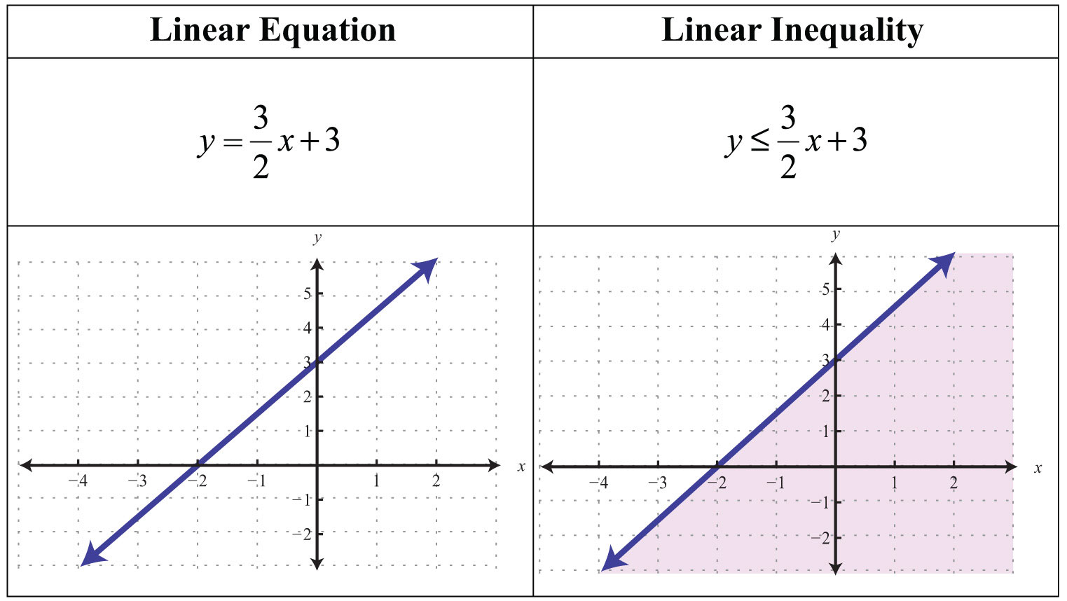
For the inequality, the line defines one boundary of the region that is shaded. This indicates that any ordered pair that is in the shaded region, including the boundary line, will satisfy the inequality. To see that this is the case, choose a few test pointsA point not on the boundary of the linear inequality used as a means to determine in which half-plane the solutions lie. and substitute them into the inequality.
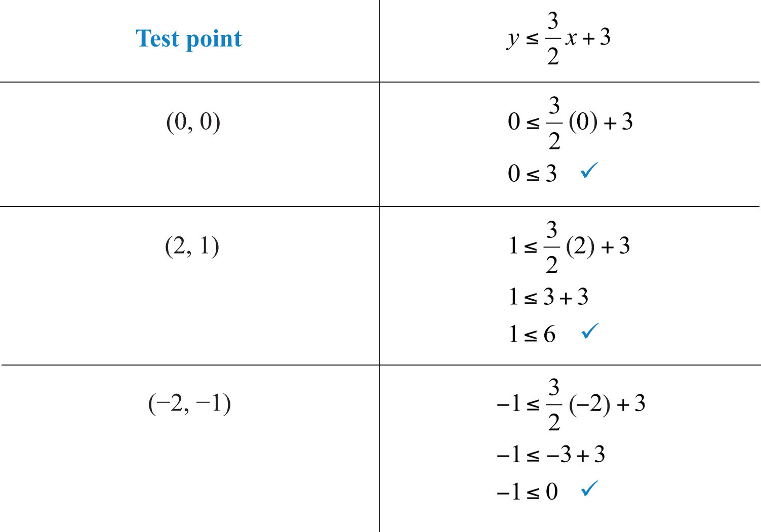
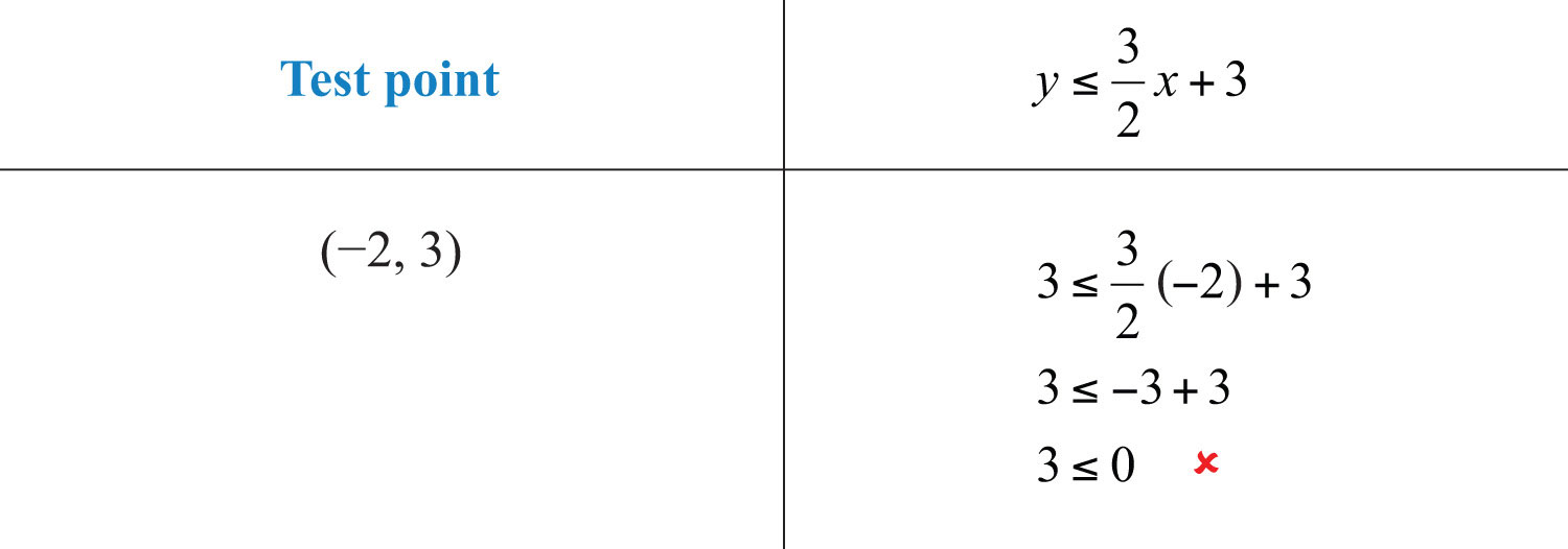
Also, we can see that ordered pairs outside the shaded region do not solve the linear inequality.
The graph of the solution set to a linear inequality is always a region. However, the boundary may not always be included in that set. In the previous example, the line was part of the solution set because of the “or equal to” part of the inclusive inequality . If we have a strict inequality , we would then use a dashed line to indicate that those points are not included in the solution set.
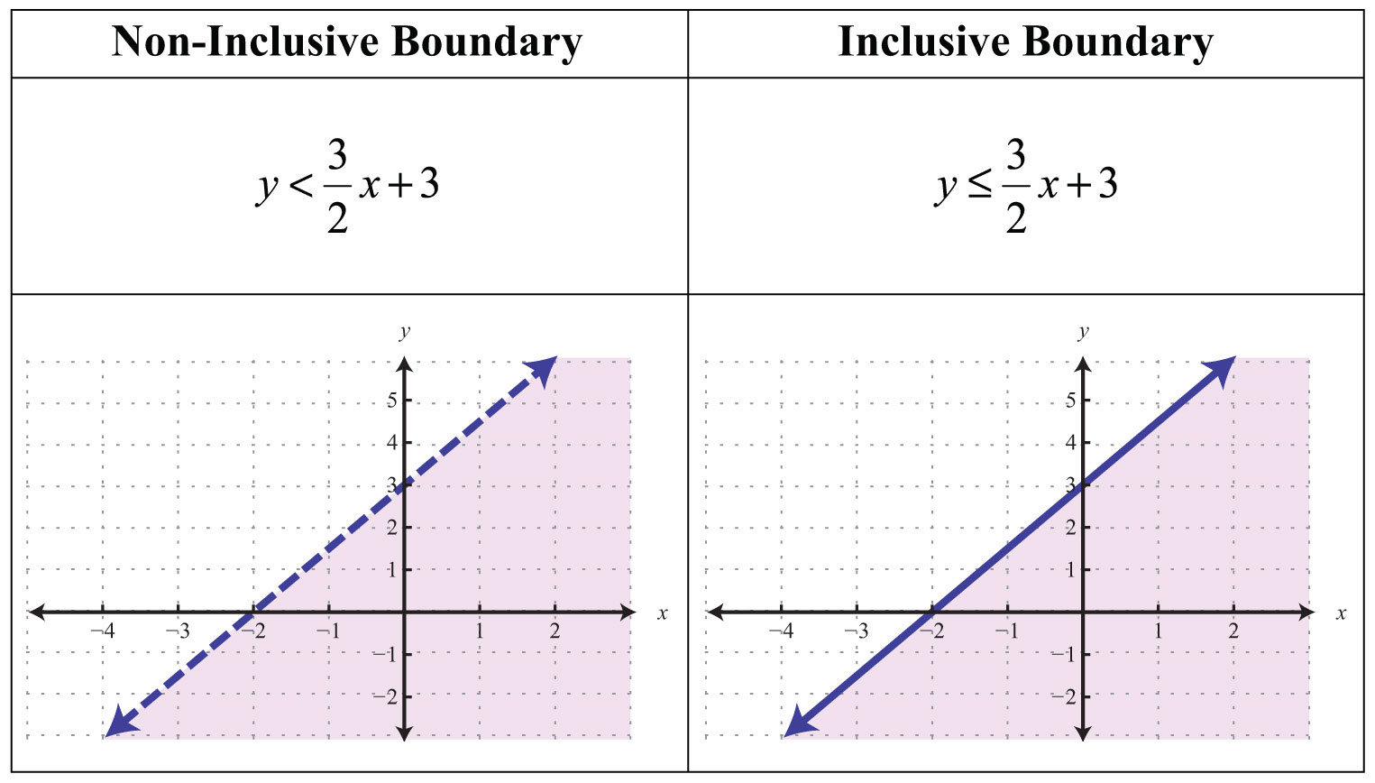
Consider the point (0, 3) on the boundary; this ordered pair satisfies the linear equation. It is the “or equal to” part of the inclusive inequality that makes it part of the solution set.

So far, we have seen examples of inequalities that were “less than.” Now consider the following graphs with the same boundary:
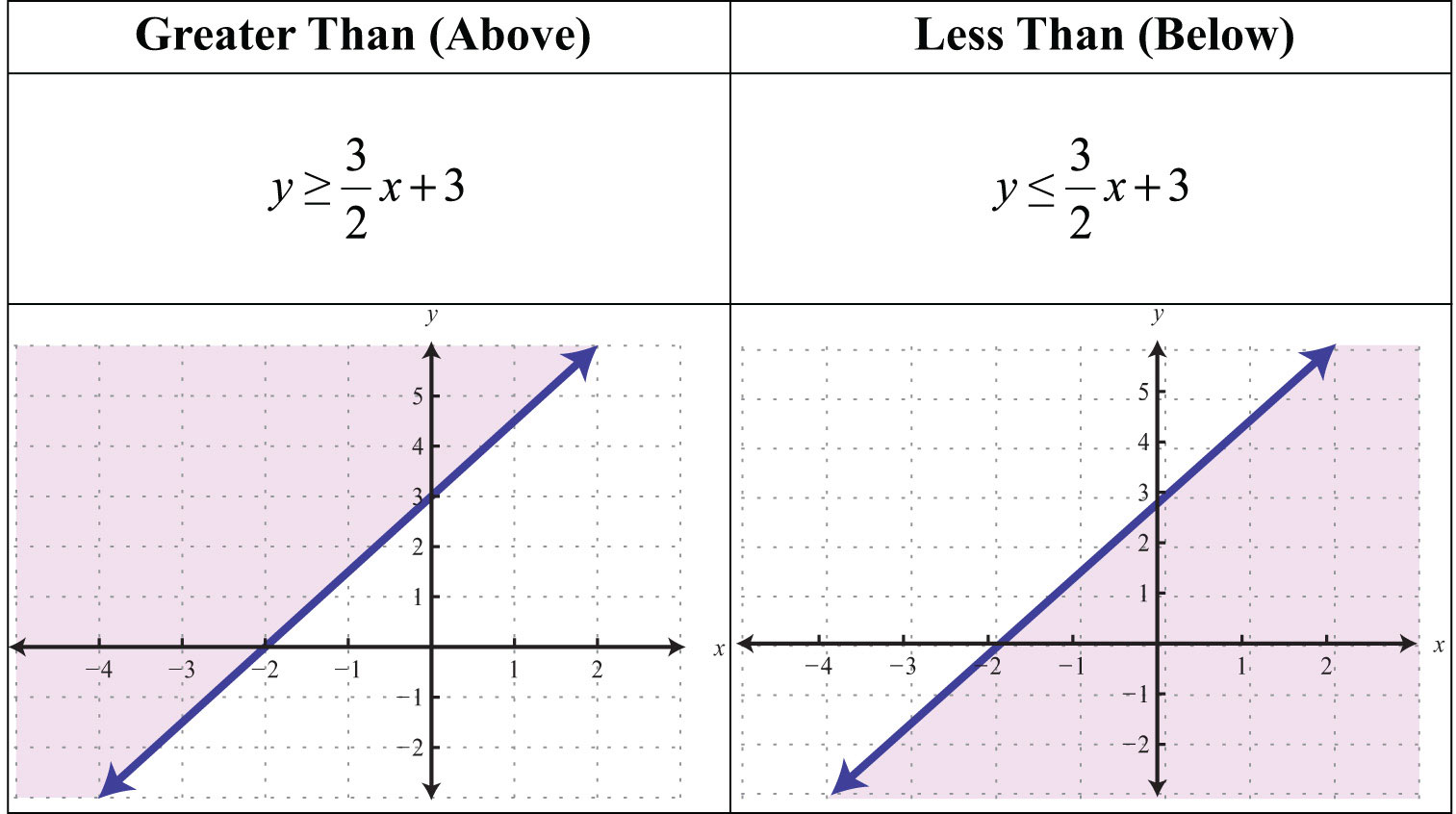
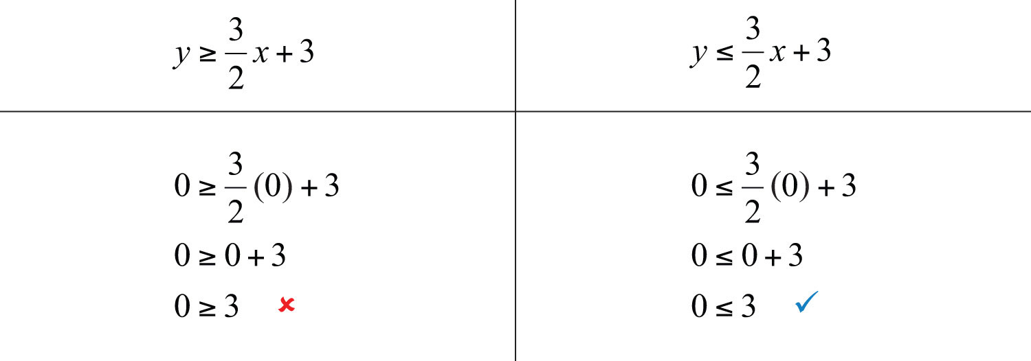
Given the graphs above, what might we expect if we use the origin (0, 0) as a test point?
Try this! Which of the ordered pairs (−2, −1), (0, 0), (−2, 8), (2, 1), and (4, 2) solve the inequality ?
Answer: (−2, 8) and (4, 2)
Video Solution
(click to see video)Graphing Solutions to Linear Inequalities
Solutions to linear inequalities are a shaded half-plane, bounded by a solid line or a dashed line. This boundary is either included in the solution or not, depending on the given inequality. If we are given a strict inequality, we use a dashed line to indicate that the boundary is not included. If we are given an inclusive inequality, we use a solid line to indicate that it is included. The steps for graphing the solution set for an inequality with two variables are outlined in the following example.
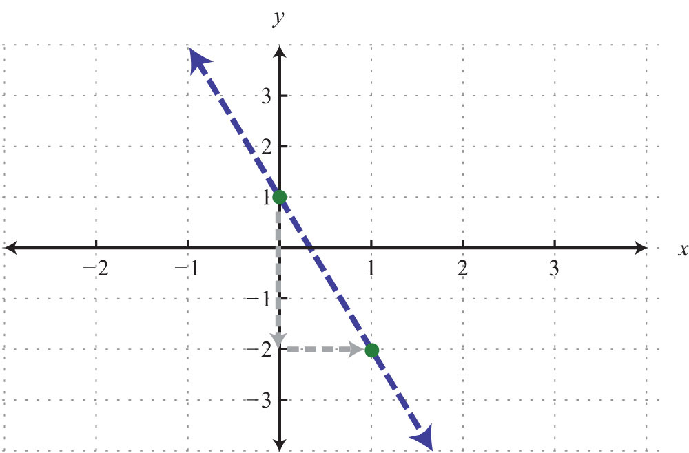
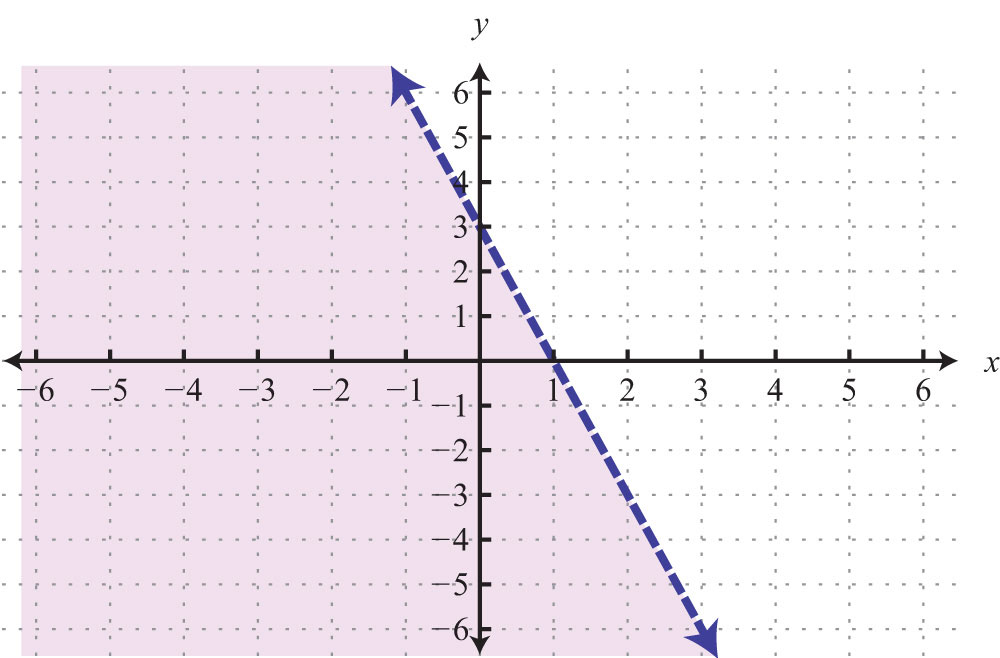
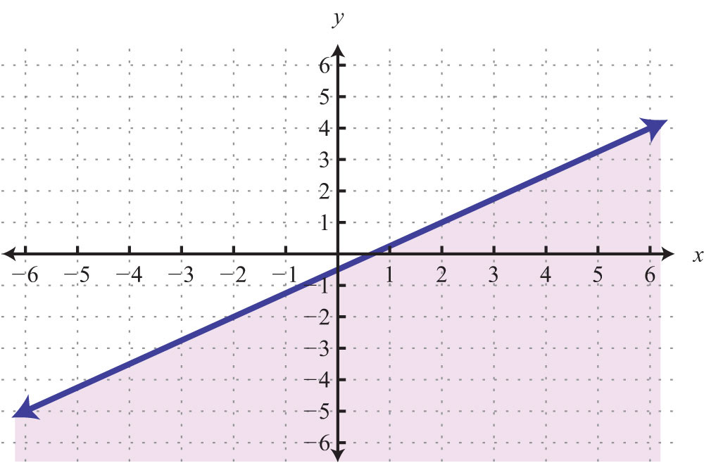
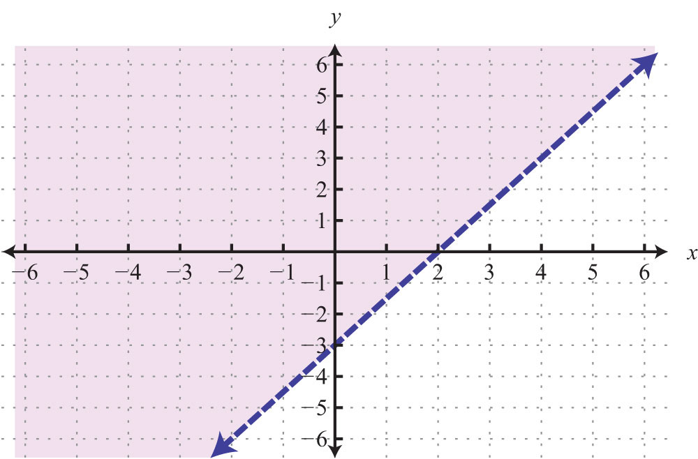
Example 1: Graph the solution set: .
Solution:
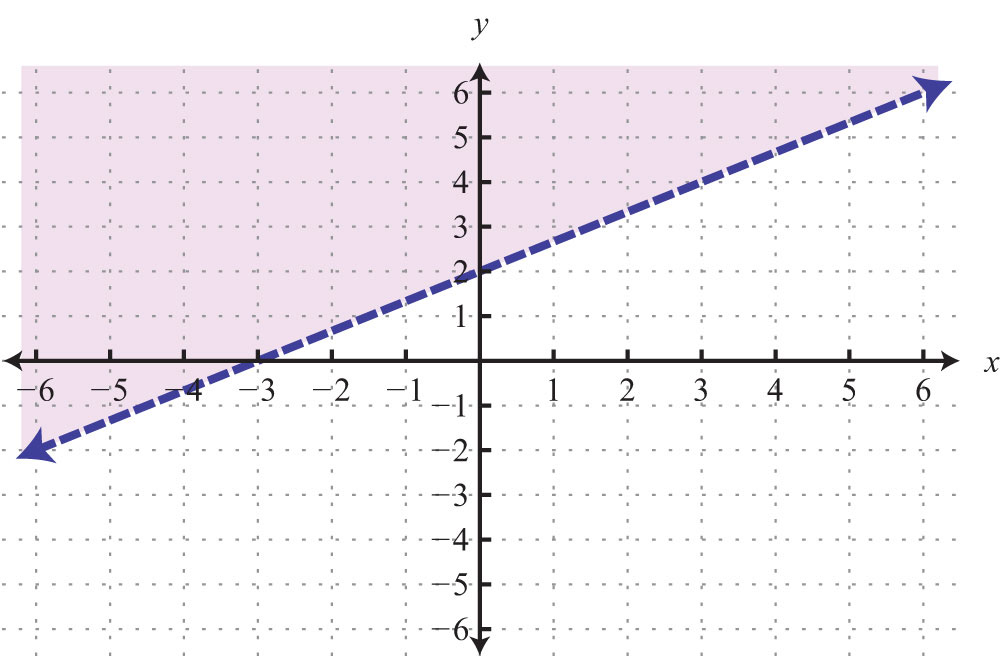
Step 1: Graph the boundary line. In this case, graph a dashed line because of the strict inequality. By inspection, we see that the slope is and the y-intercept is (0, 1).
Step 2: Test a point not on the boundary. A common test point is the origin (0, 0). The test point helps us determine which half of the plane to shade.
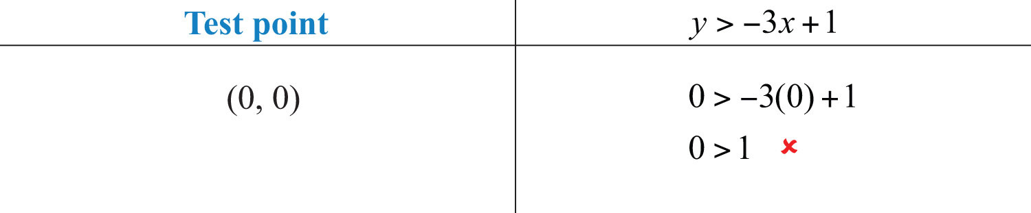
Step 3: Shade the region containing the solutions. Since the test point (0, 0) was not a solution, it does not lie in the region containing all the ordered pair solutions. Therefore, shade the half of the plane that does not contain this test point. In this case, shade above the boundary line.
Answer:
Consider the problem of shading above or below the boundary line when the inequality is in slope-intercept form. If , then shade above the line. If , then shade below the line. Use this with caution; sometimes the boundary is given in standard form, in which case these rules do not apply.
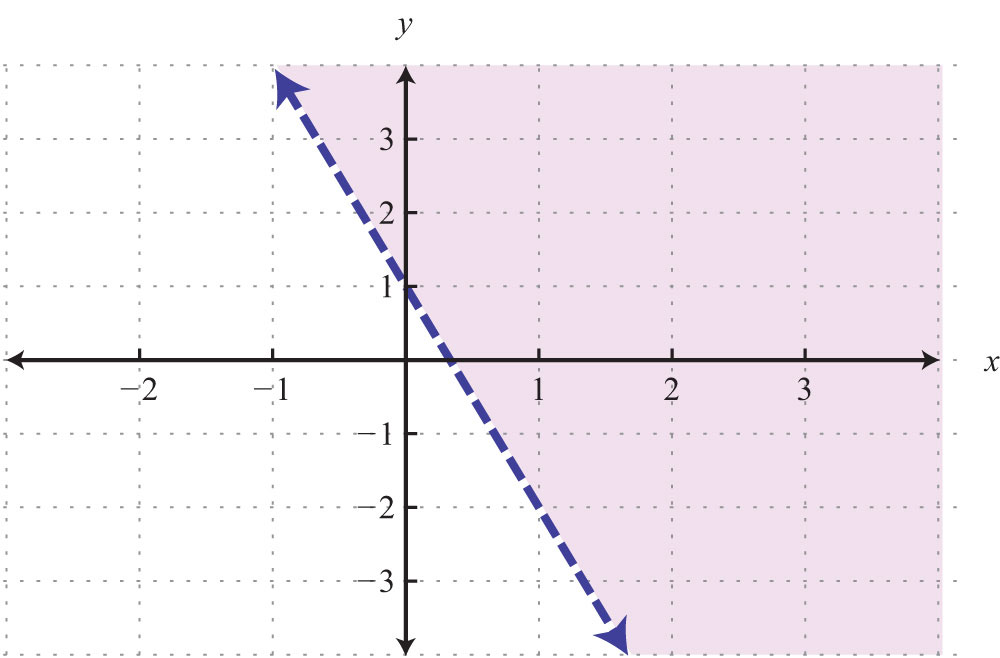
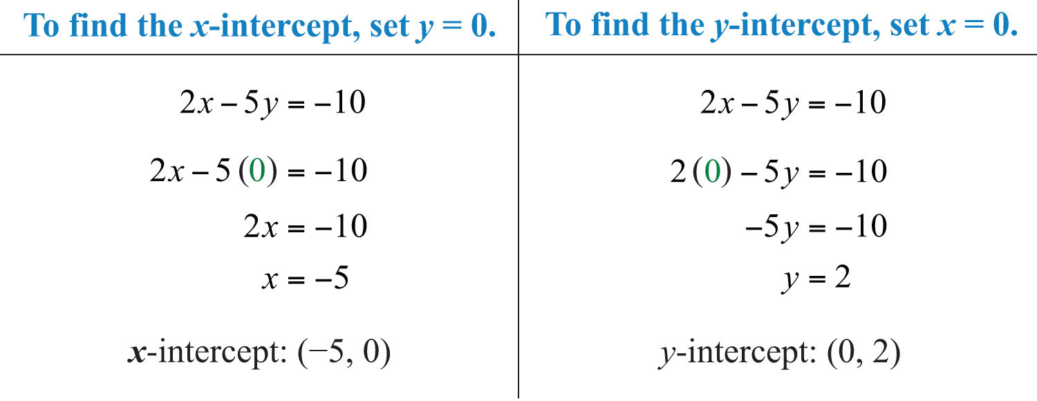
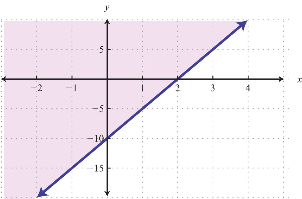
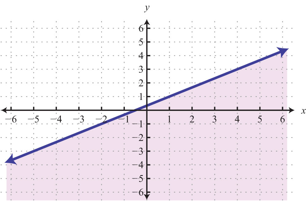
Example 2: Graph the solution set: .
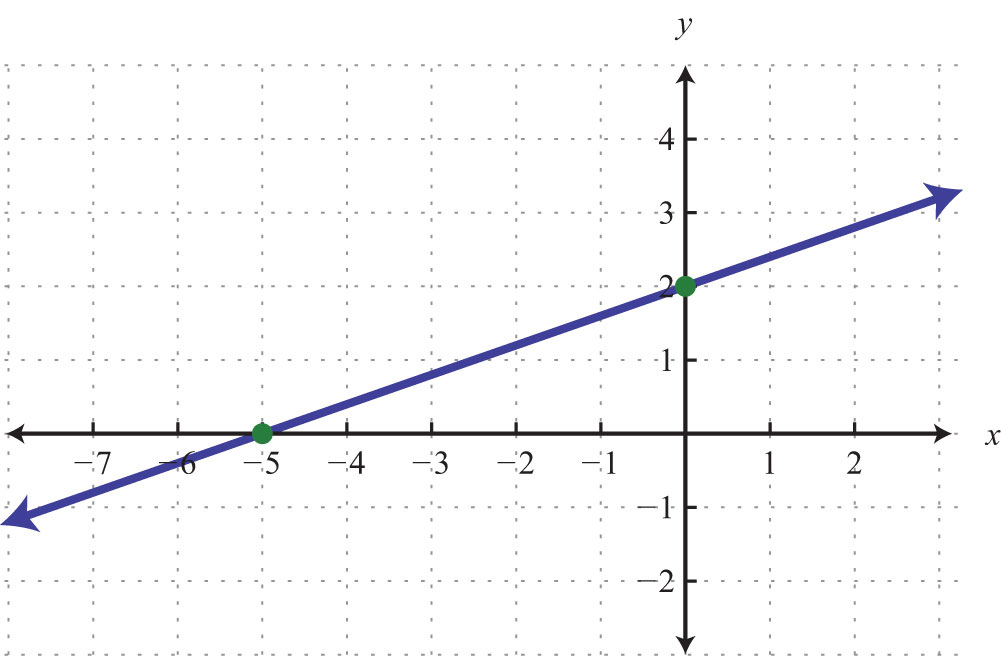
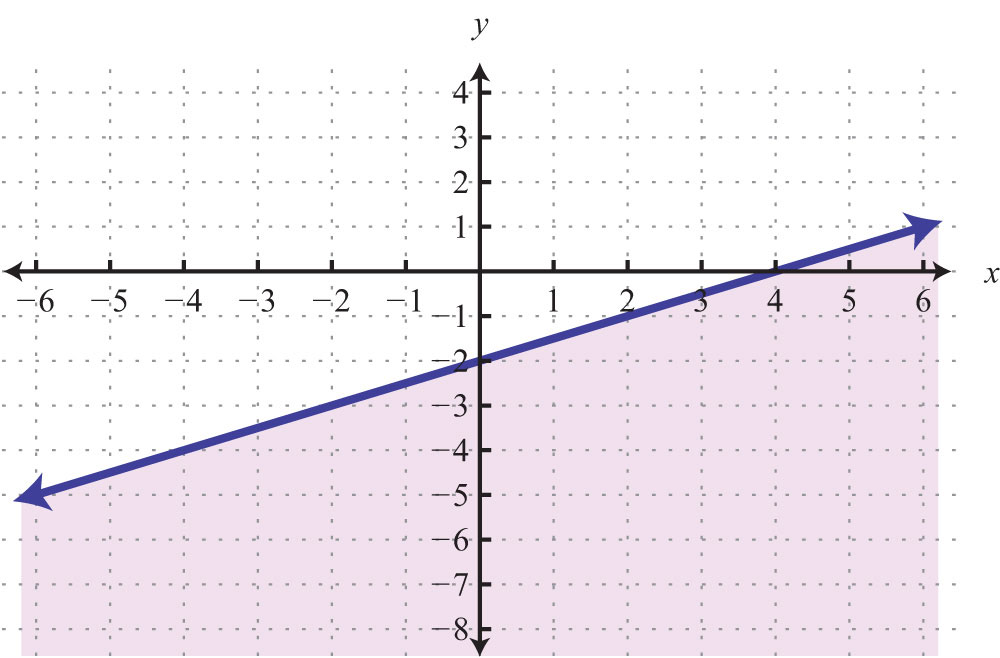
Solution: Here the boundary is defined by the line . Since the inequality is inclusive, we graph the boundary using a solid line. In this case, graph the boundary line using intercepts.
Next, test a point; this helps decide which region to shade.
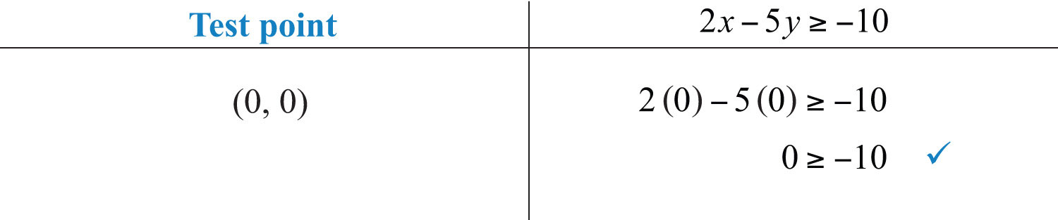
Since the test point is in the solution set, shade the half of the plane that contains it.
Answer:
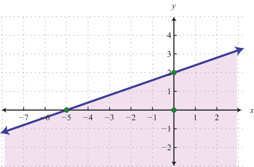
In this example, notice that the solution set consists of all the ordered pairs below the boundary line. This may be counterintuitive because of the original ≥ in the inequality. This illustrates that it is a best practice to actually test a point. Solve for y and you see that the shading is correct.
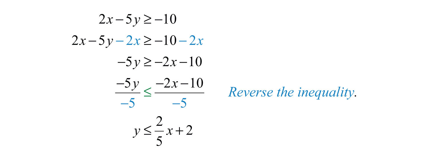
In slope-intercept form, you can see that the region below the boundary line should be shaded. An alternate approach is to first express the boundary in slope-intercept form, graph it, and then shade the appropriate region.
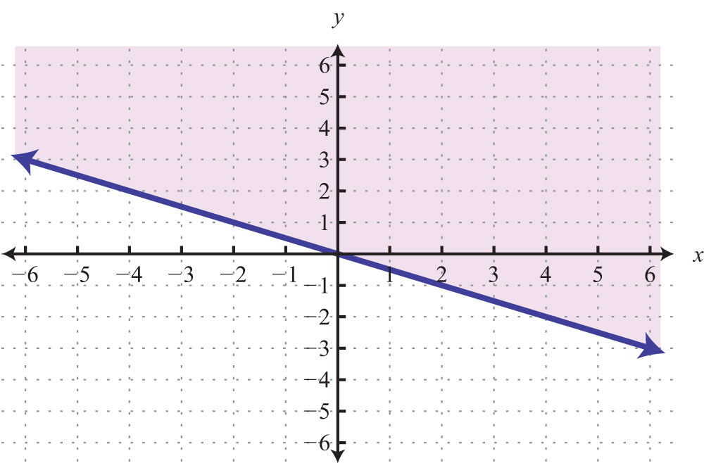
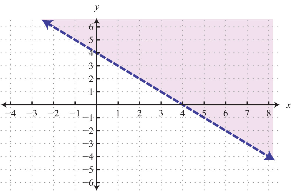
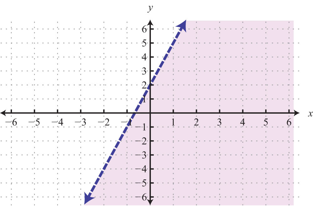
Example 3: Graph the solution set: .
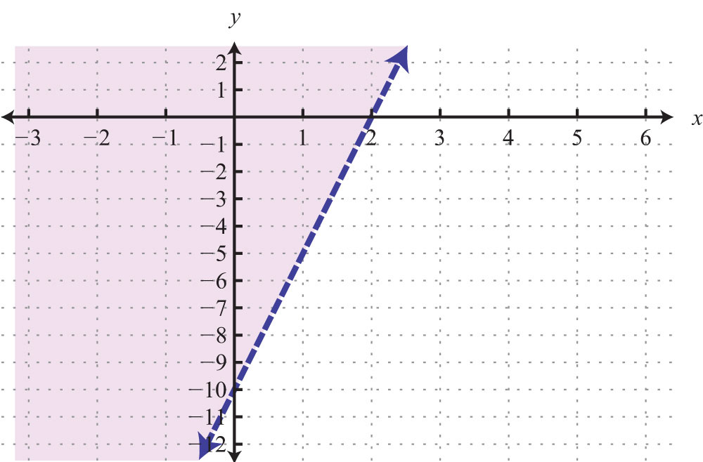
Solution: First, graph the boundary line with a dashed line because of the strict inequality.
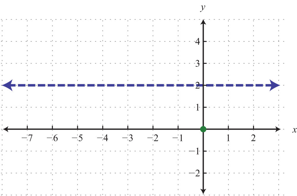
Next, test a point.

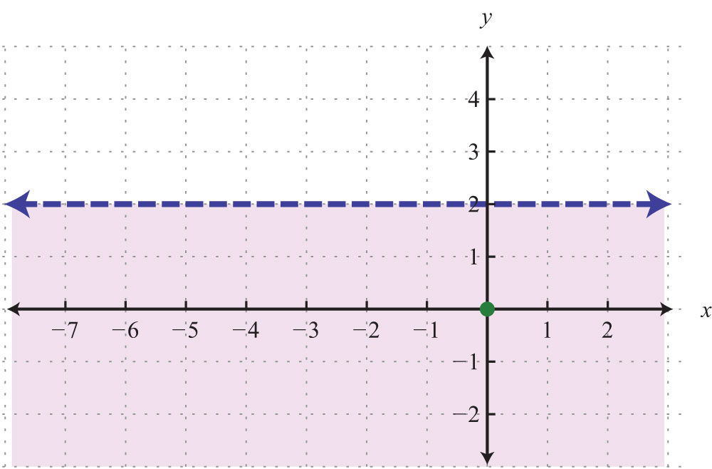
In this case, shade the region that contains the test point.
Answer:
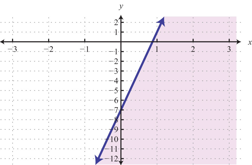
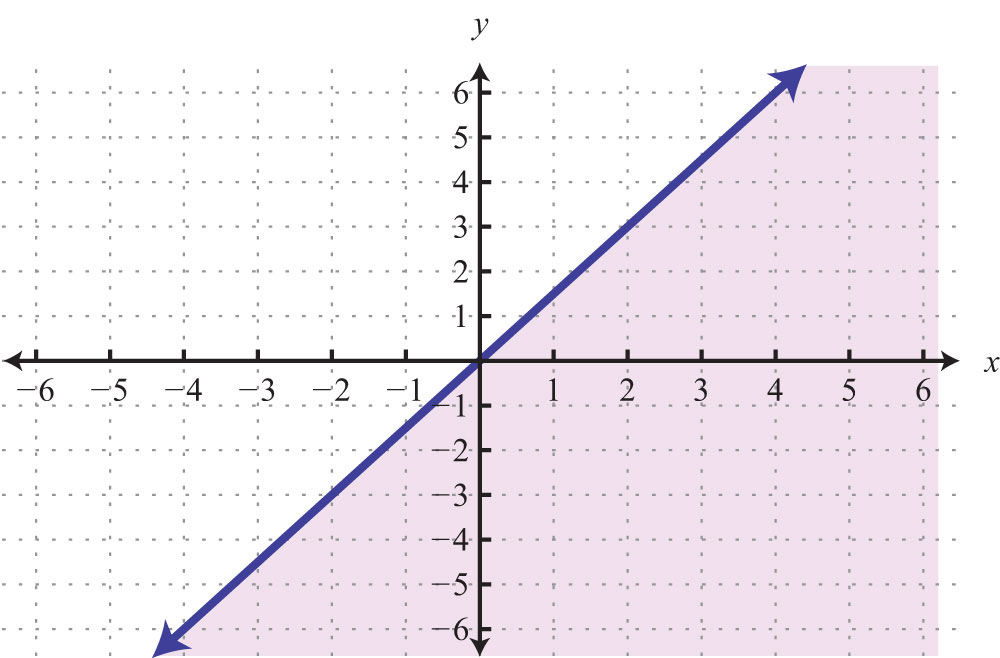
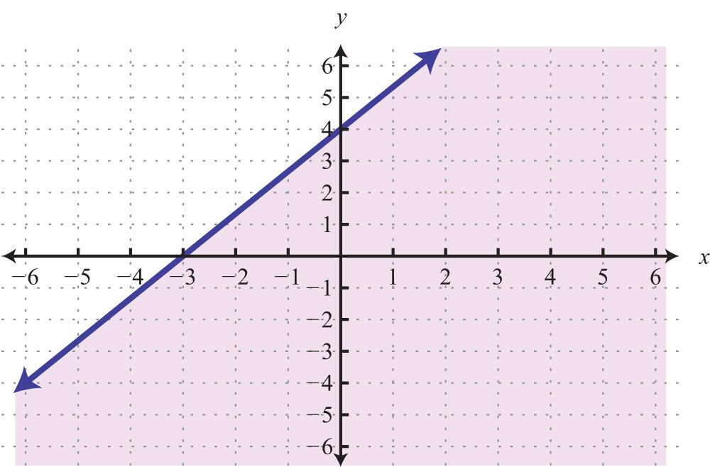
Try this! Graph the solution set: .
Answer:
Video Solution
(click to see video)Key Takeaways
- Linear inequalities with two variables have infinitely many ordered pair solutions, which can be graphed by shading in the appropriate half of a rectangular coordinate plane.
- To graph the solution set of a linear inequality with two variables, first graph the boundary with a dashed or solid line depending on the inequality. If given a strict inequality, use a dashed line for the boundary. If given an inclusive inequality, use a solid line. Next, choose a test point not on the boundary. If the test point solves the inequality, then shade the region that contains it; otherwise, shade the opposite side.
- When graphing the solution sets of linear inequalities, it is a good practice to test values in and out of the solution set as a check.
Topic Exercises
Part A: Solutions to Linear Inequalities (Two Variables)
Is the ordered pair a solution to the given inequality?
1. ; (0, 0)
2. ; (0, −2)
3. ; (6, 5)
4. ; (−3, −8)
5. ;
6. ; (−2, −1)
7. ; (0, 0)
8. ; (5, −3)
9. ; (−3, −1)
10. ; (0, 7)
Part B: Graphing Solutions to Linear Inequalities
Graph the solution set.
11.
12.
13.
14.
15.
16.
17.
18.
19.
20.
21.
22.
23.
24.
25.
26.
27.
28.
29.
30.
31.
32.
33.
34.
35.
36.
37.
38.
39.
40.
41.
42.
43. Write an inequality that describes all points in the upper half-plane above the x-axis.
44. Write an inequality that describes all points in the lower half-plane below the x-axis.
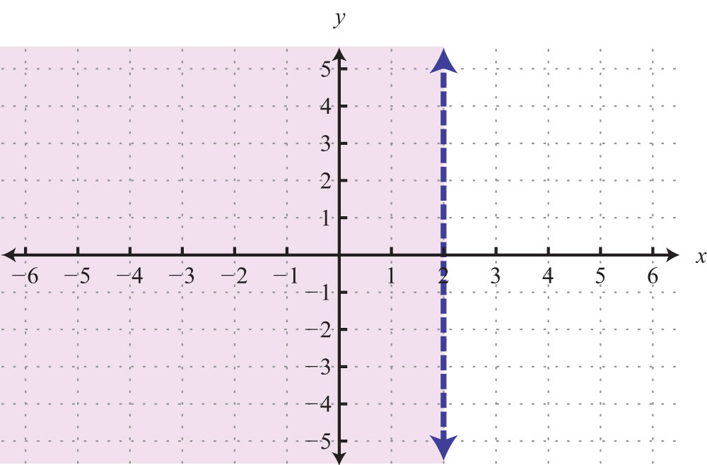
45. Write an inequality that describes all points in the half-plane left of the y-axis.
46. Write an inequality that describes all points in the half-plane right of the y-axis.
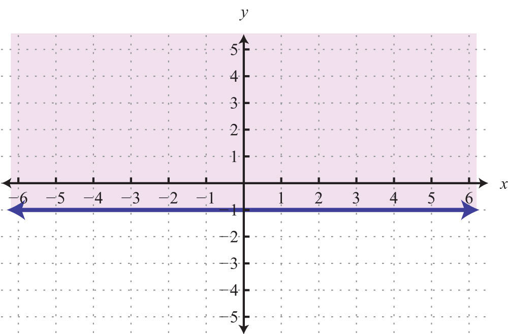
47. Write an inequality that describes all ordered pairs whose y-coordinates are at least 2.
48. Write an inequality that describes all ordered pairs whose x-coordinate is at most 5.
Answers
1: Yes
3: Yes
5: Yes
7: No
9: Yes
11:
13:
15:
17:
19:
21:
23:
25:
27:
29:
31:
33:
35:
37:

39:
41:
43:
45:
47: