Direct Materials Variance Analysis

10.3 Direct Materials Variance Analysis

Learning Objective

Calculate and analyze direct materials variances.

Question: In the dialogue at the beginning of the chapter, the president of Jerry’s Ice Cream was concerned about significant cost overruns for direct materials. We cannot simply explain these costs by saying that “we paid too much for materials” or “too many materials were used in production.” Variances must be calculated to identify the exact cause of the cost overrun. What variances are used to analyze the difference between actual direct material costs and standard direct material costs?

Answer: The difference between actual costs and standard (or budgeted) costs is typically explained by two separate variances: the materials price variance and materials quantity variance. The materials price varianceThe difference between actual costs for materials purchased and budgeted costs based on the standards. is the difference between actual costs for materials purchased and budgeted costs based on the standards. The materials quantity varianceThe difference between the actual quantity of materials used in production and budgeted materials that should have been used in production based on the standards. is the difference between the actual quantity of materials used in production and budgeted materials that should have been used in production based on the standards.

To this point, we have provided the data for Jerry’s Ice Cream necessary to calculate standard costs. However, you must also have the actual materials cost and materials quantity data to calculate the variances described previously. The actual data for the year are as follows:

Sales volume	210,000 units
Direct materials purchased	440,000 pounds
Cost of direct materials purchased	$1.20 per pound
Direct materials used in production	399,000 pounds

Recall from Figure 10.1 "Standard Costs at Jerry’s Ice Cream" that the direct materials standard price for Jerry’s is $1 per pound, and the standard quantity of direct materials is 2 pounds per unit. Figure 10.4 "Direct Materials Variance Analysis for Jerry’s Ice Cream" shows how to calculate the materials price and quantity variances given the actual results and standards information. Review this figure carefully before moving on to the next section where these calculations are explained in detail.

Figure 10.4 Direct Materials Variance Analysis for Jerry’s Ice Cream

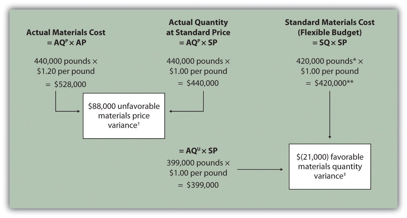
Note: AQ^P = Actual quantity of materials purchased. AP = Actual price of materials. AQ^U = Actual quantity of materials used in production. SP = Standard price of materials. SQ = Standard quantity of materials for actual level of activity.

*Standard quantity of 420,000 pounds = Standard of 2 pounds per unit × 210,000 actual units produced and sold.

**$420,000 standard direct materials cost matches the flexible budget presented in Note 10.18 "Review Problem 10.2".

^† $88,000 unfavorable materials price variance = $528,000 – $440,000. Variance is unfavorable because the actual price of $1.20 is higher than the expected (budgeted) price of $1.

^‡ $(21,000) favorable materials quantity variance = $399,000 – $420,000. Variance is favorable because the actual quantity of materials used in production of 399,000 pounds is lower than the expected (budgeted) quantity of 420,000 pounds.

Direct Materials Price Variance Calculation

Question: The materials price variance answers the question, did we spend more or less on direct materials than expected? If the variance is unfavorable, we spent more than expected. If the variance is favorable, we spent less than expected. How is the materials price variance calculated?

Answer: As shown in Figure 10.4 "Direct Materials Variance Analysis for Jerry’s Ice Cream", the materials price variance is the difference between the actual quantity of materials purchased at the actual price and the actual quantity of materials purchased at the standard price:

Key Equation

Materials price variance = (AQ^P × AP) – (AQ^P × SP)

\begin{matrix} Materials price variance & = ({AQ}^{P} \times AP) - ({AQ}^{P} \times SP) \\ = (44 0,000 \times $1 . 20) - (44 0,000 \times $1 .00) \\ = $88, 000 unfavorable \end{matrix}

Alternative Calculation. Since we are holding the actual quantity constant and evaluating the difference between actual price and standard price, the materials price variance calculation can be simplified as follows:

Key Equation

Materials price variance = (AP – SP) × AQ^P

\begin{matrix} Materials price variance & = (AP - SP) \times {AQ}^{P} \\ = ($1 . 20 - $1 .00) \times 44 0,000 \\ = $88, 000 unfavorable \end{matrix}

Note that both approaches—the direct materials price variance calculation and the alternative calculation—yield the same result.

When labeling the variances calculated in this chapter, notice that all positive variances are unfavorable and all negative variances are favorable (i.e., unfavorable cost variances increase expected costs and favorable cost variances decrease expected costs). As you calculate variances, you should think through the variance to confirm whether it is favorable or unfavorable. For example, the materials price variance calculation presented previously shows the actual price paid for materials was $1.20 per pound and the standard price was $1. Clearly, this is unfavorable because the actual price was higher than the expected (budgeted) price.

Direct Materials Quantity Variance Calculation

Question: The materials quantity variance answers the question, did we use more or fewer direct materials in production than expected? If the variance is unfavorable, we used more than expected. If the variance is favorable, we used fewer than expected. How is the materials quantity variance calculated?

Answer: As shown in Figure 10.4 "Direct Materials Variance Analysis for Jerry’s Ice Cream", the materials quantity variance is the difference between the actual quantity of materials used in production at the standard price and the standard quantity of materials allowed at the standard price:

Key Equation

Materials quantity variance = (AQ^U × SP) – (SQ × SP)

\begin{matrix} Materials quantity variance & = ({AQ}^{U} \times SP) - (SQ \times SP) \\ = (399, 000 \times $1 .00) - (42 0,000 \times $1 .00) \\ = ($21, 000) favorable \end{matrix}

The standard quantity of 420,000 pounds is the quantity of materials allowed given actual production. For Jerry’s Ice Cream, the standard quantity of materials per unit of production is 2 pounds per unit. Thus the standard quantity (SQ) of 420,000 pounds is 2 pounds per unit × 210,000 units produced and sold.

Alternative Calculation. Since we are holding the standard price constant and evaluating the difference between actual quantity used and standard quantity, the materials quantity variance calculation can be simplified as follows:

Key Equation

Materials quantity variance = (AQ^U – SQ) × SP

\begin{matrix} Materials quantity variance & = ({AQ}^{U} - SQ) \times SP \\ = (399, 000 - 42 0,000) \times $1 .00 \\ = ($21, 000) favorable \end{matrix}

Note that both approaches—the direct materials quantity variance calculation and the alternative calculation—yield the same result.

The materials quantity variance calculation presented previously shows the actual quantity used in production of 399,000 pounds is lower than the expected (budgeted) quantity of 420,000 pounds. Clearly, this is favorable because the actual quantity used was lower than the expected (budgeted) quantity.

Possible Causes of Direct Materials Variances

Question: The managerial accountant at Jerry’s Ice Cream will likely investigate the cause of the unfavorable materials price variance of $88,000. This will lead to discussions with the purchasing department. What might have caused the $88,000 unfavorable materials price variance?

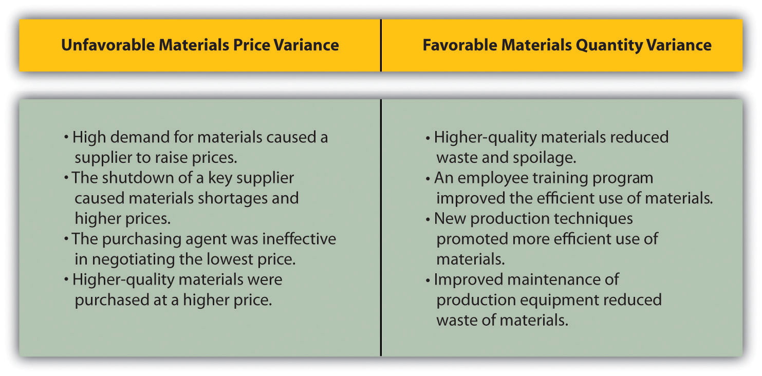
Answer: The left panel of Figure 10.5 "Possible Causes of Direct Materials Variances for Jerry’s Ice Cream" contains some possible explanations for this variance.

Figure 10.5 Possible Causes of Direct Materials Variances for Jerry’s Ice Cream

Whatever the cause of this unfavorable variance, Jerry’s Ice Cream will likely take action to improve the cost problem identified in the materials price variance analysis. This is why we use the term control phase of budgeting to describe variance analysis. Through variance analysis, companies are able to identify problem areas (material costs for Jerry’s) and consider alternatives to controlling costs in the future.

Question: Jerry’s Ice Cream might also choose to investigate the $21,000 favorable materials quantity variance. Although this could be viewed as good news for the company, management may want to know why this favorable variance occurred. What might have caused the $21,000 favorable materials quantity variance?

Answer: The right panel of Figure 10.5 "Possible Causes of Direct Materials Variances for Jerry’s Ice Cream" contains some possible explanations for this variance.

Notice how the cause of one variance might influence another variance. For example, the unfavorable price variance at Jerry’s Ice Cream might have been a result of purchasing high-quality materials, which in turn led to less waste in production and a favorable quantity variance. This also might have a positive impact on direct labor, as less time will be spent dealing with materials waste.

Note 10.26 "Business in Action 10.2" illustrates just how important it is to track direct materials variances accurately.

Business in Action 10.2

The Effect of Rising Materials Costs on Auto Suppliers

In the first six months of 2004, steel prices increased 76 percent, from $350 a ton to $617 a ton. For auto suppliers that use hundreds of tons of steel each year, this had the unexpected effect of increasing expenses and reducing profits. For example, a major producer of automotive wheels had to reduce its annual earnings forecast by $10,000,000 to $15,000,000 as a result of the increase in steel prices.

Most auto part suppliers operate with very small margins. GR Spring and Stamping, Inc., a supplier of stampings to automotive companies, was generating pretax profit margins of about 3 percent prior to the increase in steel prices. Profit margins have been cut in half since steel prices began rising.

These thin margins are the reason auto suppliers examine direct materials variances so carefully. Any unexpected increase in steel prices will likely cause significant unfavorable materials price variances, which will lead to lower profits. Auto part suppliers that rely on steel will continue to scrutinize materials price variances and materials quantity variances to control costs, particularly in a period of rising steel prices.

Source: Brett Clanton, “Steel Costs Slam Auto Suppliers,” The Detroit News, June 29, 2004, http://www.detnews.com.

Clarification of Favorable Versus Unfavorable

Question: Why are variances labeled favorable or unfavorable?

Answer: The terms favorable and unfavorable relate to the impact the variance has on budgeted operating profit. A favorable varianceA variance that has a positive impact on operating profit. has a positive impact on operating profit. An unfavorable varianceA variance that has a negative impact on operating profit. has a negative impact on operating profit. Companies using a standard cost system ultimately credit favorable variances and debit unfavorable variances to income statement accounts. The appendix to this chapter describes this process in further detail.

Key Takeaway

Standard costs are used to establish the flexible budget for direct materials. The flexible budget is compared to actual costs, and the difference is shown in the form of two variances. The materials price variance focuses on the price paid for materials, and it is defined as the difference between the actual quantity of materials purchased at the actual price and the actual quantity of materials purchased at the standard price. The materials quantity variance focuses on the quantity of materials used in production. It is defined as the difference between the actual quantity of materials used in production and budgeted materials that should have been used in production based on the standards.

Review Problem 10.3

Carol’s Cookies expected to use 1.5 pounds of direct materials to produce 1 unit (batch) of product at a cost of $2 per pound. Actual results are in for last year, which indicates 390,000 batches of cookies were sold. The company purchased 640,000 pounds of materials at $1.80 per pound and used 624,000 pounds in production.

Calculate the materials price and quantity variances using the format shown in Figure 10.4 "Direct Materials Variance Analysis for Jerry’s Ice Cream".
Use the alternative approach to calculating the materials price and quantity variances, and compare the result to the result in part 1. (Hint: the variances should match.)
Suggest several possible reasons for the materials price and quantity variances.

Solution to Review Problem 10.3

As shown in the following, the materials price variance is $(128,000) favorable, and the materials quantity variance is $78,000 unfavorable.

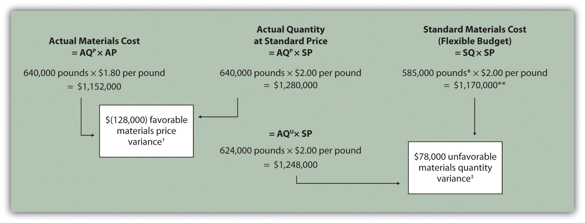
Note: AQ^P = Actual quantity of materials purchased. AP = Actual price of materials. AQ^U = Actual quantity of materials used in production. SP = Standard price of materials. SQ = Standard quantity of materials for actual level of activity.

*Standard quantity of 585,000 pounds = Standard of 1.5 pounds per unit × 390,000 actual units produced and sold.

**$1,170,000 standard direct materials cost matches the flexible budget presented in Note 10.18 "Review Problem 10.2", part 2.

^† $(128,000) favorable materials price variance = $1,152,000 – $1,280,000. Variance is favorable because the actual price of $1.80 is lower than the expected (budgeted) price of $2

^‡ $78,000 unfavorable materials quantity variance = $1,248,000 – $1,170,000. Variance is unfavorable because the actual quantity of materials used in production of 624,000 pounds is higher than the expected (budgeted) quantity of 585,000 pounds.
Alternative direct materials variance calculations:
$\begin{matrix} Materials price variance & = (AP - SP) \times {AQ}^{P} \\ = ($1 . 80 - $2 .00) \times 640,000 \\ = ($128,000) favorable (same as part 1) \end{matrix}$ $\begin{matrix} Materials quantity variance & = ({AQ}^{U} - SQ) \times SP \\ = (624,000 - 585,000) \times $2 .00 \\ = $78,000 unfavorable (same as part 1) \end{matrix}$
Possible causes of favorable materials price variance are
- The supplier had excess materials on hand and lowered prices to sell off inventory;
- New suppliers entered the market, which resulted in an excess supply of materials and lower prices;
- Carol’s Cookies’ purchasing agent is a strong negotiator and was able to negotiate lower prices than anticipated;
- Lower-quality materials were purchased at a lower price.
Possible causes of unfavorable materials quantity variance are
- Lower-quality materials resulted in more waste and spoilage;
- New, inexperienced employees were hired, resulting in more waste;
- Old equipment breaking down caused an increased amount of waste.